To normalize earnings for a cyclical stock, average the company's operating margin across a full business cycle, then apply that mid-cycle margin to current revenue. Deduct interest and tax, and divide by the current diluted share count. The result estimates sustainable earning power rather than a single year's outcome. Use it as the earnings base for multiples and as the starting level for a DCF. Averaging margins beats averaging past earnings per share because it scales with the company's current size.
Why the latest year misleads for cyclical stocks
Cyclical businesses sell demand that customers can postpone. Mining equipment, memory chips, new houses, airline seats, steel, and oil investment all expand and contract with the economy or with their own industry's capacity cycle. Revenue swings, and operating leverage amplifies the effect. A large fixed cost base makes operating income move much further than revenue, so margins expand and compress with the cycle.
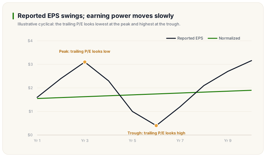
That amplification breaks the trailing multiple as a screening signal. At the top of the cycle, earnings are inflated, so the price-to-earnings ratio looks low and the stock screens as cheap. At the bottom, earnings collapse or turn negative, the ratio looks enormous or meaningless, and the stock screens as expensive. Experienced analysts treat this inversion as a standing feature of deep cyclicals. The multiple often says buy at the peak and avoid at the trough, which is close to the opposite of the economics underneath.
The same distortion flows into any method that consumes a single year of earnings. An EV/EBITDA multiple applied to peak EBITDA overstates enterprise value in exact proportion to the overstatement in the base figure. A DCF that projects from a trough base either undervalues the business or forces the whole rebound into the growth rates. The error is upstream of the method. Fixing it means fixing the earnings input first, and that is what normalization does.
What are normalized earnings?
Normalized earnings estimate the profit a company would report in the middle of its cycle, under ordinary conditions, at its current size. The concept extends a cleanup step most analysts already run. Stripping one-time items such as asset sales or litigation settlements, as covered in the broader stock valuation methods guide, removes accidents from a single year. Cycle normalization goes further. It removes the position of that year inside the business cycle, which no amount of one-time-item cleanup can see.
The logic has a long pedigree. Aswath Damodaran's paper on valuing cyclical and commodity companies frames the problem directly. For these firms the base-year choice dominates the valuation, so the analyst should replace it with a normalized measure of earnings or margins. At the index level, the same smoothing instinct produced the cyclically-adjusted PE ratio, which divides a market's price by its ten-year average of real earnings. The CAPE calculation methodology is designed for market indices, though, and its authors say so. Company-level normalization is the single-stock counterpart, and it has to work with a shorter history, one business model, and no offsetting constituents.
A normalized figure is an estimate, and it should be labeled as one. It will be wrong in any specific year by design. Its job is to be less wrong on average than the reported number it replaces.
How do you locate a company in its cycle?
Normalization starts with a position fix. Before averaging anything, establish whether current results sit near a peak, near a trough, or somewhere in between. Four kinds of evidence do most of the work.
First, compare current margins with the company's own long history. Pull eight to twelve years of income statements from the filings on SEC EDGAR and compute the operating margin for each year. A current margin near the historical high is peak evidence regardless of what management calls it. Second, compare revenue with its long-run trend. Revenue far above trend usually means the industry is over-earning, and capacity additions are on the way.
Third, look at industry-level indicators. For industrial cyclicals, the Federal Reserve's industrial production index shows where aggregate output sits relative to its own history. For commodity producers, compare the commodity price with the marginal cost of new supply; prices far above that cost attract the investment that eventually ends the party. Fourth, watch capital behavior. Aggressive capacity expansion, large acquisitions, and buybacks concentrated at high prices are peak behavior. Idled plants, dividend cuts, and equity raises cluster at troughs.
One warning applies to every cycle: the phrase "this time is different" appears most often at the top. Management commentary written at a peak tends to explain why the peak is the new normal. The filings record what was said in the last cycle, and reading them is a cheap vaccine.
Figure 1. Reported earnings through a cycle against normalized earning power
The trailing multiple inverts for deep cyclicals: it looks cheapest at the earnings peak and most expensive at the trough, while mid-cycle earning power moves slowly.
How to calculate normalized earnings step by step
The margin method is the workhorse. It anchors the estimate to the company's current scale, which matters because most businesses grow across a cycle. Averaging past earnings per share instead would anchor the estimate to the smaller company of five or ten years ago. Here is the sequence.
-
Collect eight to twelve years of revenue and operating income, enough to span at least one full cycle for that industry.
-
Compute the operating margin for each year, then average the margins across the window. Check that the window contains both a peak and a trough.
-
Apply the average margin to current-year revenue. The product is normalized operating income.
-
Deduct interest expense at its current level, since capital structure is a present-day fact rather than a cyclical one.
-
Apply the current statutory tax rate to reach normalized net income, or a normalized effective rate if the company's rate differs from it persistently.
-
Divide by the current diluted share count for normalized earnings per share. Use today's share count even for the averaged margin, because yesterday's share count belongs to a company that no longer exists.
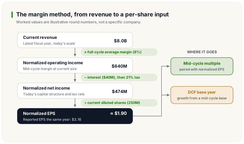
A worked example makes the size of the correction visible. The figures are illustrative round numbers, not a specific company. Suppose an industrial equipment maker reports $8.0 billion of revenue and a 13 percent operating margin in the current year. Its operating margins over the past ten years, most recent year first, ran 13, 11, 8, 4, 2, 5, 9, 12, 10, and 6 percent. They average 8 percent. Normalized operating income is $8.0 billion times 8 percent, or $640 million. Deduct $40 million of interest to reach $600 million pre-tax, apply a 21 percent tax rate, and normalized net income is $474 million. Across 250 million diluted shares, normalized EPS is about $1.90.
The reported numbers tell a different story. Reported operating income is $1.04 billion, which becomes $790 million of net income and $3.16 of EPS on the same interest, tax, and share inputs. At a $38 share price, the stock trades at 12 times reported earnings and 20 times normalized earnings. The company screens as cheap only because the snapshot was taken at the top of its cycle.
Figure 2. From current revenue to a normalized valuation input
The margin method: a full-cycle average margin applied to current revenue, carried down to a per-share figure on today's capital structure.
Two refinements are worth knowing. If revenue itself sits far above or below trend, normalize revenue first and then apply the mid-cycle margin, since a peak includes both price and volume effects. And if the company discloses clean segment data, normalize segment by segment. A stable service segment averaged together with a violent equipment segment produces a mid-cycle margin that describes neither.
How do normalized earnings feed a multiple or a DCF?
For relative valuation, pair the normalized earnings estimate with a mid-cycle multiple. The pairing matters as much as the estimate. Market multiples move against the cycle: they compress at earnings peaks and expand at troughs, because prices anticipate the turn before the income statement reports it. Applying an expanded trough-year multiple to normalized earnings re-imports the recovery you already built into the estimate. The company's own multiple history across a full cycle is the cleanest anchor. Apply the same normalization to every peer before comparing, because two cyclicals measured at different points in their cycles are not comparable on reported numbers. Where trough earnings turn negative and the earnings multiple stops working, practitioners switch to price-to-book or enterprise value per unit of capacity as the temporary anchor. The same discipline extends to enterprise-value multiples, where the EBITDA figure needs normalizing before any multiple touches it.
For a DCF, normalized earning power anchors the base year. A forecast that starts at a trough forces the rebound into the growth assumptions, where it hides; one that starts at a peak extends conditions that are already ending. Setting the starting level at mid-cycle, then expressing growth as the path from that base, keeps the model honest. Cash flow needs the same treatment as earnings. Capital expenditure and working capital swing with the cycle too, so anchor the capex-to-sales ratio at its full-cycle average before reading any free cash flow figure as sustainable. The InvestViable Valuator runs the DCF calculation from three explicit inputs: the cash flow growth path, the discount rate, and the terminal growth rate. Whether the growth path starts from a sustainable base is the analyst's judgment, and normalization is how that judgment gets made. The remaining inputs deserve the same scrutiny; the DCF inputs checklist covers how to verify each one, and its margin questions are the audit-side counterpart of the method built here.
Whichever method consumes the estimate, present the output as a range. A normalized figure carries estimation error in the window choice, the margin average, and the cycle read. Ranges make that error visible instead of hiding it behind one decimal-pointed number.
Where normalization breaks
Normalization assumes the past cycle describes the future one. Four situations break that assumption.
Structural decline is the expensive failure. When demand is shrinking for secular reasons (substitution, regulation, or technology), historical margins are not coming back, and a mid-cycle average flatters the business. The averaging arithmetic works perfectly and the answer is still wrong. The tell is in the driver, covered in the FAQ below: volumes that fall across successive cycles and recovery peaks that keep coming in lower.
Supercycles are the mirror-image failure. Some commodity and capital-goods cycles run longer than any reasonable averaging window. A ten-year average taken inside one long upswing is then itself a peak number wearing a disguise. If the industry's investment cycle plausibly runs longer than your data, widen the window where history allows, or lean harder on the marginal-cost logic for the commodity in question.
Short histories defeat the method mechanically. A company that listed five years ago, a spin-off, or a business transformed by a large acquisition has no clean full-cycle record. Industry-level margin history can substitute, applied with judgment about how the specific company differs from the average producer.
Accounting changes contaminate the window quietly. A margin series that spans a major standard change mixes two definitions of the same line. The lease-accounting change under IFRS 16 is the classic example. It split operating lease cost into depreciation and interest, lifting operating margins mid-series; US GAAP filers were largely untouched on that line. Check comparability across the window before trusting the average, and restate where the filings give you enough to do it.
One caveat sits outside the arithmetic. A leveraged cyclical has to survive the trough before mid-cycle earnings matter, so check debt maturities and covenant headroom before trusting any normalized figure.
When you cannot decide between the cyclical and structural readings, run both. Value the company on the normalized estimate and on a structurally impaired one, and let the two results define the range. The disagreement between them is information, and averaging it away would discard exactly the thing you learned.
How to apply this
Treat normalization as a standing habit for any business whose margins have a visible wave in them. Pull the long margin history and fix the company's position in its cycle. Build the mid-cycle estimate with the margin method, and only then let a multiple or a DCF see the number. Write down the window and the average you used, so the estimate can be audited when the cycle turns.
Sector screens are a natural starting point, since cyclicality clusters by industry. The energy and industrials slices of the Stock Universe collect the fundamentals for two of the classic cyclical sectors in one place. From there, the normalization work runs on the filings, and the valuation methods from the core methods guide consume the estimate you built.
Rebuild the estimate once a year, after the annual filing lands, and after any acquisition or divestiture large enough to change the margin structure. Reported earnings will disagree with your normalized figure in most individual years. That is the estimate working as designed. The disagreement only becomes a warning when it stops cycling and starts trending.
InvestViable does not publish buy or sell recommendations on individual securities. All analysis is based on public financial data and a transparent methodology. The Investment Score formula is proprietary; the inputs and what the score evaluates are documented.