How to calculate cyclically-adjusted PE: a methodology guide

What CAPE actually does

The cyclically-adjusted PE ratio evaluates the long-term valuation of an equity market index. Standard trailing PE distorts during economic transitions because one or two unusual years of earnings dominate the denominator. CAPE addresses that distortion at the cost of slower responsiveness.

Robert Shiller developed the metric to address that problem. The ten-year inflation-adjusted earnings average smooths out the noise of the standard business cycle: when companies experience temporary profit spikes or severe one-off losses, the ten-year window dilutes those anomalies. The result is a denominator that approximates normal-conditions earning power rather than current-conditions earning power.

The metric is designed for long-run forecasting, not short-window timing. Campbell and Shiller's 1988 research paper established the dividend-forecasting framework: a moving average of real earnings is a stable input for forecasting future cash flows to shareholders. The popular "CAPE predicts ten-year returns" framing comes from later empirical work (Campbell and Shiller's 1998 follow-up) and from Shiller's Irrational Exuberance; the original 1988 paper was about dividend forecasting, not return prediction per se.

Mechanically, the ten-year window is what determines how CAPE behaves: it adjusts slowly, it integrates information from the previous economic cycle, and it produces a smooth signal even when underlying earnings are volatile. Whether that smoothing produces a useful interpretation of the current market is a separate question. For the methodology to be applied consistently, the analyst needs to pin down the formula, the data sources, and the input choices first. What CAPE measures and where it fails for modern markets takes up the interpretive question.

Step-by-step formula for cyclically-adjusted PE

Standard PE uses one year of earnings data, which makes it susceptible to temporary distortions. CAPE demands a more rigorous ten-year lookback.

1. Identify the current price level of the stock market index.

2. Adjust the current index price for inflation to establish the real stock price (in some reference-year dollars).

3. Collect the index's earnings per share data for the past ten years.

4. Adjust each year of historical earnings for inflation to match current purchasing power.

5. Calculate the simple arithmetic average of the ten years of inflation-adjusted earnings.

6. Divide the real stock price by the ten-year average real earnings per share.

The result is CAPE (also written PE10). Skipping the inflation-adjustment step is a common error: if older earnings are left in nominal dollars, they appear artificially low relative to the current price, which inflates the final ratio.

Financial data collection

Ten full years of earnings reports capture at least one complete economic cycle. The calculation requires an inflation adjustment that relies on the Consumer Price Index published by the BLS, or equivalently the CPIAUCSL series in FRED. The adjustment maintains purchasing-power parity across eras: a dollar of earnings reported a decade ago represented more real economic activity than a dollar reported today. Without this step, the ten-year average understates real economic output and the resulting CAPE reading is biased downward.

The GAAP versus non-GAAP earnings choice

This is the input choice that drives most of the divergence between CAPE readings published by different sources. Some analysts use Generally Accepted Accounting Principles (GAAP) earnings, which include all expenses and one-time write-offs. Others use non-GAAP operating earnings, which exclude extraordinary items and produce a smoother baseline.

GAAP earnings drop sharply during recessions because companies write down impaired assets, which drags the ten-year average down and pushes the resulting CAPE ratio higher during the subsequent recovery years. Non-GAAP earnings remain more stable across the cycle and typically produce a lower CAPE reading. This distinction explains why one source might report a current CAPE near 33 while another shows 31 for the same market on the same date. Shiller's own dataset uses strictly reported GAAP earnings, the most conservative choice, and the reason Shiller's published CAPE typically runs slightly higher than alternative versions.

Reliable historical metrics sources

Most analysts do not build a CAPE dataset from scratch. Several retail-facing data aggregators publish pre-calculated CAPE readings alongside Robert Shiller's own Yale dataset, which remains the primary source most other providers ultimately derive from. InvestViable provides valuation context for analysts wanting a single environment for both market-level metrics and stock-level work. Standard readings often vary slightly across providers because of the GAAP-versus-non-GAAP question and because of small differences in how each source rebases the inflation series. The methodological differences typically explain a one-to-two-point gap in the headline number; analysts should verify the methodology footnotes before comparing readings across sources.

Macro inputs that affect the calculation

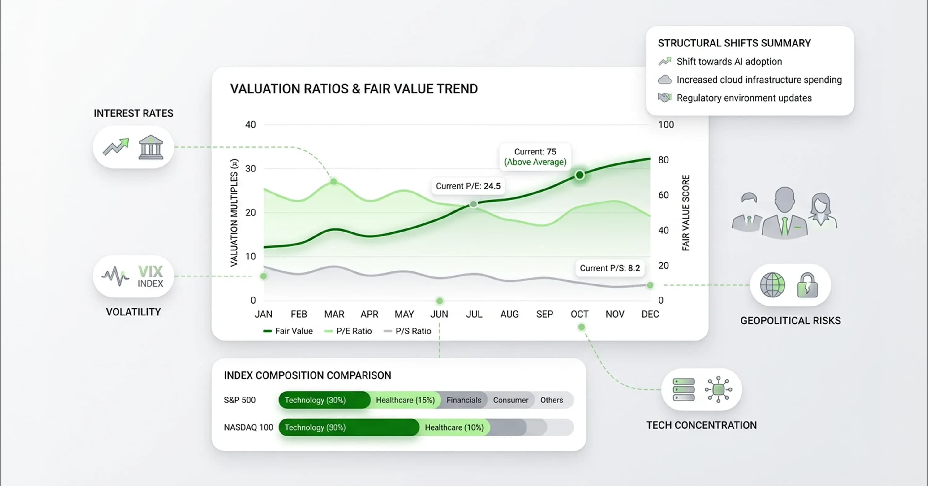
The calculation itself is deterministic, but two macro inputs determine whether the resulting number is comparable to historical CAPE data: the prevailing real interest rate regime and the index's earnings-series continuity across structural breaks.

During the 1970s inflationary period, real interest rates rose sharply and compressed market valuations. Market participants demanded higher real yields, which pushed CAPE down into single digits. The modern low-inflation era operates under different conditions. The empirical baseline an analyst uses for comparison matters as much as the calculation itself. CFA Institute's analysis of structurally elevated CAPE levels documents this regime dependency.

The calculation also requires the index's earnings series to be reasonably continuous across the ten-year window. Major accounting changes (FAS 142 in 2001, ASC 606 in 2018, ASC 842 in 2019) shift the definition of reported earnings mid-window, which means the ten-year denominator mixes earnings calculated under two different accounting regimes. The Shiller dataset documents these breaks but doesn't restate prior years. Analysts running CAPE on shorter regional indices with less continuity (emerging markets, sector indices) must check the earnings-series continuity explicitly before treating the calculated value as comparable to U.S. long-run history.

These are inputs to the calculation, not interpretations of the output. The methodology is robust to both, provided the analyst documents which regime and which accounting basis the result was computed under.

Index composition as a calculation input

The index composition is part of the calculation, not an interpretation layer on top of it. CAPE on a cap-weighted index aggregates earnings from constituents in proportion to their market capitalisation; CAPE on an equal-weighted index aggregates them in equal proportion. The two calculations produce different numbers from the same underlying companies.

The S&P 500's largest constituents represented roughly 40% of index weight at their peak in 2025. For a cap-weighted CAPE, that concentration means the calculation's denominator is materially shaped by the ten-year earnings histories of about ten companies. The denominator's composition can change meaningfully across a ten-year window as the index reweights, even though the constituent list is technically stable from quarter to quarter.

Analysts who want CAPE to reflect the broader market typically compute it three ways: the standard cap-weighted version (the headline number most sources publish), an equal-weighted version (which dilutes the concentration effect), and the median constituent's individual PE10 (which removes concentration entirely). The three calculations produce different values, and the methodological decision about which version to use is upstream of any interpretation.

For company-specific valuation work that bypasses index-level aggregation entirely, transparent valuation tools, comparable-based analysis, and the stock market value calculation formulas workflow apply directly to individual issuers rather than to the aggregate.

Formula variants: P-CAPE and beyond

Financial researchers have proposed variants of the standard formula to address modern corporate behavior. Companies now return capital to shareholders through stock buybacks rather than only through traditional dividends, and the standard CAPE formula does not adjust for this shift. Researchers developed the payout-adjusted cyclically-adjusted PE (P-CAPE) metric in response. During recent market cycles, the P-CAPE has tracked roughly 19% above the standard metric. This gap traces directly to the 2010s shift toward buybacks over dividends, as Bunn and Shiller documented in their 2014 NBER paper.

The payout-adjusted version better reflects modern corporate finance, but analysts must decide whether the added mathematical complexity justifies the marginal accuracy gain. For most calculation purposes, the standard ten-year average still provides enough precision to calibrate portfolio expectations. Minor formula adjustments rarely change the broader forecast meaningfully, and the more significant interpretive question (whether CAPE is the right metric for the current market regime at all) is independent of which variant the analyst chose.

This article's scope ends at producing the calculated value. The interpretive question (why elevated CAPE readings don't reliably predict short-term corrections, and how to integrate the metric into portfolio decisions without overreacting) lives in a companion piece: What CAPE measures and where it fails for modern markets. For the broader context an analyst should place any single CAPE reading into, see valuation ranges and fundamental analysis frameworks.

How to use this calculation

The calculation reduces to five decisions an analyst should document for any CAPE number they cite. First, the formula itself: the standard PE10 ratio with a ten-year inflation-adjusted earnings denominator. Second, the earnings basis: GAAP-reported (Shiller's choice and the most conservative) versus operating earnings (smoother, typically produces lower readings). Third, the data source: Shiller's Yale dataset as the primary, with secondary aggregators verified against it. Fourth, the calculation-context inputs: real interest rate regime, earnings-series continuity across structural accounting breaks, and the index aggregation method (cap-weighted, equal-weighted, or median). Fifth, the formula variant: standard PE10 or the P-CAPE payout-adjusted version for portfolios where buyback intensity materially shifts the cash-distribution profile.

Each of these is a calculation input, not a portfolio signal. The interpretive question (what to do with the resulting number in a portfolio context) lives in the companion piece on what CAPE measures and where it fails for modern markets.

The next step is applying the calculated value to portfolio decisions at the individual stock level. InvestViable provides valuation tools for moving from market-level CAPE readings to assessing whether specific stocks trade at a discount to their intrinsic value.