
Valuation sensitivity analysis measures how much your estimated value changes when you change an input. Run a one-way test on each uncertain input, flexing it across a defensible range while holding the rest at the base case, then rank the inputs by how far each moves the value. That ranking, shown as a tornado chart, tells you which assumptions to verify hardest. A two-way table then shows how the two dominant inputs interact. The deliverable is never a single number. It is a range whose width reflects how much the valuation had to assume, and that width sets the margin of safety you demand.
What valuation sensitivity analysis is
Valuation sensitivity analysis is the disciplined version of a question every analyst asks anyway: what if I am wrong about this? A model turns a set of assumptions into a single value. That value looks authoritative, but it inherits all the uncertainty of the inputs behind it. Sensitivity analysis makes the uncertainty visible by changing an input, holding the others still, and recording the new value. Do this across the inputs that could reasonably be different, and the fragile point estimate becomes a map of how the valuation behaves.
Valuation sensitivity analysis
A structured test that varies one or more inputs of a valuation model across plausible ranges and records the effect on the estimated value, in order to identify which assumptions the conclusion depends on and how wide the range of defensible values really is.
The reason this matters is that inputs do not contribute equally. Aswath Damodaran's work on probabilistic approaches to valuation frames sensitivity analysis, scenario analysis, and simulation as the standard tools for dealing with the estimation risk baked into every model. The point estimate is where the pillar guide to valuation methods ends; sensitivity analysis is what you do with that estimate before you trust it. Without it, you cannot tell whether your fair value is robust or whether it hangs entirely on one optimistic assumption.
Which inputs to stress-test, and how far
Before you stress-test your assumptions, confirm they are worth stressing. Two conditions have to hold: the input must carry real uncertainty, and it must be capable of moving the answer. The current cash balance is known, so leave it fixed. Next year's revenue growth is a forecast, and in most models it moves the value a lot, so it belongs in the test. Running a sensitivity analysis is the natural next step after you audit the DCF inputs for defensibility. First you check the inputs are sound; then you find out which ones the valuation leans on.
In a discounted cash flow model, three inputs almost always earn a place in the test. They are the discount rate, the terminal growth rate, and the near-term free cash flow or margin path. In a multiple-based valuation, it is the chosen multiple and the normalized earnings base. The discount rate deserves particular attention because it is both uncertain and powerful, which is why choosing it well warrants its own WACC walkthrough. The market's risk-free anchor for that rate is the 10-year Treasury yield published by the Federal Reserve via FRED. It shifts over time, so a rate that looked right last year may not this year.
How far you flex each input is a judgment, not a fixed rule. Calibrate the band to how well the input is known. A mature company's long-run growth might justify half a percentage point either side of the base case; a young company's near-term growth could warrant several points. The discount rate is commonly flexed by about a percentage point in each direction. Using one arbitrary width for every input, say plus or minus ten percent across the board, defeats the purpose. It hides the fact that some assumptions are far shakier than others. The band should reflect the genuine range a reasonable analyst could defend for that specific business.
One-way sensitivity: isolate one input at a time
A one-way analysis changes a single input across its plausible band while holding everything else at the base case. It answers a precise question: taken on its own, how much does this input move the value? To make the mechanics concrete, take a simplified single-stage model where value equals next year's free cash flow divided by the discount rate minus the perpetual growth rate. The figures below are illustrative round numbers, not a specific company. Base case: free cash flow of $100 million, a discount rate of 9 percent, and perpetual growth of 3 percent. That gives a value of $100m / (0.09 − 0.03), or about $1,667 million.
Now flex each input on its own. Move the discount rate from 8 to 10 percent, holding growth at 3 percent. The value ranges from $2,000 million down to about $1,429 million, a swing of $571 million. Flex free cash flow by ten percent either way and the value moves between $1,500 million and $1,833 million, a swing of $333 million. Flex the terminal growth rate from 2.5 to 3.5 percent and the value moves between about $1,538 million and $1,818 million, a swing of $280 million. Rank those swings and you have a tornado chart: the widest bar is the input that matters most.
Figure 1. A tornado chart ranks inputs by their effect on value
Each bar shows how far the estimated value moves when one input is flexed across its plausible band, with the rest held at the base case. The widest bar is where the valuation is most fragile.
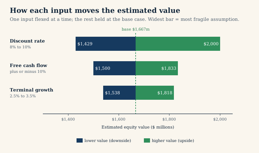
The ranking is the payoff, but it pays to be precise about what a tornado bar measures. Each bar reflects two things at once: how far the value moves per unit of change in the input, and how wide a band that input plausibly ranges over. In this single-stage model, the discount rate and terminal growth are symmetric. The discount rate leads only because its defensible band is wider, a full point either side; a mature firm's long-run growth earns a narrower band. Flex both over the same band and they would move the value equally. That is exactly why the calibration in the previous section matters: the ranking is only meaningful when each band reflects the genuine uncertainty in that input. When one input clearly leads a tornado built on honest bands, you have found the assumption your conclusion truly rests on.
Two-way sensitivity: flex two inputs together
A one-way test isolates each input, but real uncertainty rarely arrives one variable at a time. A two-way analysis flexes the two most important inputs together across a grid, showing the value at every combination. Using the same illustrative model, put the discount rate down the rows and the terminal growth rate across the columns. Each cell is $100m divided by the discount rate minus the growth rate. Reading the two together matters because they often move in the same direction. A business whose prospects are dimming tends to justify both a higher discount rate and a lower long-run growth rate. The grid captures that joint move; two separate one-way tests, each holding the other input fixed, would miss it.
Figure 2. A two-way table shows how the dominant inputs interact
Estimated value in $ millions at each combination of discount rate and terminal growth rate, holding free cash flow at $100m. The pessimistic and optimistic corners define the practical range.
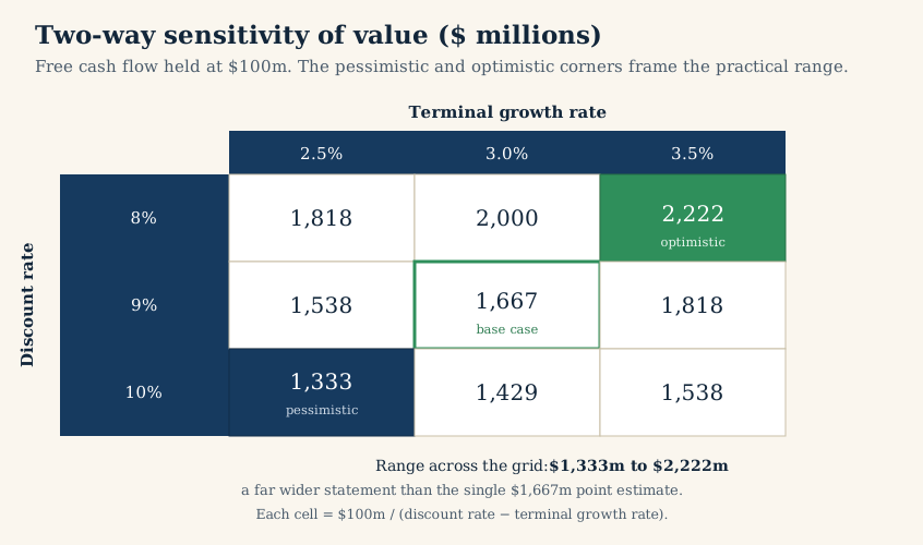
Read the corners. The optimistic corner, an 8 percent discount rate paired with 3.5 percent growth, values the business at about $2,222 million. The pessimistic corner, a 10 percent rate with 2.5 percent growth, values it at about $1,333 million. The base case sits in the middle at roughly $1,667 million. That spread, from $1,333 to $2,222 million, is a far more honest statement of what the model supports than the single base-case number is. The grid also shows interaction. A high discount rate paired with low growth is not just bad; it compounds two adverse assumptions. That corner defines the floor you should weigh most heavily.
Turning the analysis into a decision
Sensitivity analysis is only useful if it changes what you do. It feeds two decisions. The first is where to direct more research. The tornado chart names the input the valuation depends on, so that is the assumption to defend with the most evidence. If the discount rate leads, revisit the cost-of-capital build. If near-term growth leads, scrutinize the demand and margin story. Spending equal effort on every input wastes it on the ones that barely move the answer.
The second decision is the width of your valuation range, and this is where the output-as-ranges discipline becomes concrete. The corners of the two-way table are the raw material for a bear, base, and bull estimate. Presenting the result as a valuation range rather than a point keeps the uncertainty in view. A wide range is not a failure of the analysis; it is an accurate signal that the business is hard to value. Damodaran observes that valuation is least precise exactly when the potential payoff is largest. That is the reason to let the range stay wide when the inputs demand it, rather than force a false precision.
The range then calibrates the margin of safety you require. A valuation that produced a tight range from well-anchored inputs can support a purchase closer to the base case. One that produced a wide range from shaky assumptions should demand a larger discount to price, or a decision to pass. The same discipline applies when you normalize the earnings base you feed the model: the U.S. Securities and Exchange Commission's guidance on non-GAAP financial measures is a reminder that an unadjusted starting figure can quietly widen or shift the whole range.
How to apply this
Treat sensitivity analysis as a required step, not an optional flourish. Build the model and verify the inputs first. Identify the handful that carry genuine uncertainty. Run a one-way test on each, flexing it across a band calibrated to how well you know it, and rank the results in a tornado chart. Take the two inputs that dominate and build a two-way table to see how they interact and where the corners fall. Report the result as a range. Spend your remaining research time on the input that moves the value most. Size the margin of safety to the width of the range. Any tool that exposes its assumptions lets you do this directly. The InvestViable Valuator builds a discounted cash flow from three explicit inputs: the cash flow growth path, the discount rate, and the terminal growth rate. Moving one slider while watching the fair value respond is a one-way sensitivity analysis in real time. The InvestViable stock screener compares price with fair value and the Investment Score across the US universe. Check it to see where a stock sits before you start. A number that survives its own stress test is worth acting on. A number that collapses the moment you flex one assumption was never as precise as it looked.
InvestViable does not publish buy or sell recommendations on individual securities. All analysis is based on public financial data and a transparent methodology. The Investment Score formula is proprietary; the inputs and what the score evaluates are documented.