Market Concentration and What It Does to Index Valuation

What an index multiple divides, and what moves it

A capitalization-weighted index level is the sum of price times index shares across the constituents, divided by a divisor. S&P Dow Jones Indices sets out that construction in its index mathematics methodology. There the share count for each stock is scaled by an investable weight factor: the percentage of shares outstanding included in the calculation. The divisor exists to hold the index level continuous through corporate actions and rebalances. It is a scaling constant, not a valuation input.

For a multiple, the divisor cancels. Total market value over total earnings is the same number whether both sides are expressed in dollars or in index points, because a common scaling factor divides out. What survives is the ratio of two aggregates, and every question about concentration is a question about how those aggregates were built.

The two aggregates do not move together, and a published series makes the gap visible. Damodaran's S&P earnings history carries index level and index earnings by year from 1960 forward. The earnings column there is built from the index level and a published earnings yield, so a multiple taken from those two columns is that yield inverted. Read on August 27, 2026, the 2020 row shows a level of 3,756.07 against earnings of 139.76, a multiple of 26.88. The 2021 row shows 4,766.18 against 206.38, a multiple of 23.09. The index rose 26.9 percent over that year while the multiple fell 14.1 percent, because earnings rose 47.7 percent. A multiple can fall in a market that is rising, and the denominator is why. The most recent row, 2025, gives 6,845.50 over 271.52, or 25.21, against a yield column of 3.97 percent that inverts to 25.19. The two agree to within the rounding of the yield column itself. The file's own note says the most recent year's numbers include estimates for the last quarter of the year.

Three channels can therefore move an index multiple: prices, earnings, and the mix of members behind both. The earnings yield against a bond yield covers what the aggregate ratio means once computed, and how to calculate a cyclically adjusted P/E covers the denominator-smoothing choice. The third channel is the subject of the rest of this article.

The two weights a constituent carries

Write the index multiple as a ratio of sums and rearrange it. Each member's own multiple arrives carrying its share of total earnings as its coefficient, not its share of total market value.

index P/E   = total market value / total earnings
            = sum( earnings share_i x P/E_i )

index E/P   = total earnings / total market value
            = sum( market-value share_i x E/P_i )

so          market-value share_i / earnings share_i
            = P/E_i / index P/E

The last line is where the two vectors become a single testable statement. A member's market-value weight exceeds its earnings weight by exactly the factor by which its own multiple exceeds the index multiple. The two weights match only for a member priced at the index multiple.

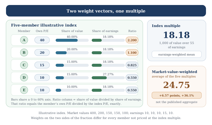
Both weights do work, in two different senses. The earnings share is the coefficient sitting on a member's own multiple. The market-value share is the fraction of the finished index multiple that member supplies. In the index below the largest member supplies 7.27 of the 18.18, and its share of the total is exactly its market-value weight of 40.00 percent.

A five-member index makes the two vectors visible at once. Market values of 400, 200, 150, 150 and 100 sum to 1,000. Earnings of 10, 10, 10, 15 and 10 sum to 55. The five multiples are 40, 20, 15, 10 and 10, and the index multiple is 1,000 over 55, or 18.18. Market-value weights run 40.00, 20.00, 15.00, 15.00 and 10.00 percent. Earnings weights run 18.18, 18.18, 18.18, 27.27 and 18.18 percent. The largest member holds 40.00 percent of the value and 18.18 percent of the earnings, a ratio of 2.200. The ratio is exactly its own multiple of 40 divided by the index multiple of 18.18.

Now weight those five multiples by market value, the calculation most readers would reach for. It returns 24.75, which is 6.57 points and 36.1 percent above the index multiple of 18.18. That number is not wrong so much as it answers a different question. Index providers publish the aggregate ratio, not this average of the ratios, and the two are built on different weights. They are not interchangeable inputs to a comparison.

One caveat belongs on the denominator, and it matters as soon as a real membership is used. A member with small positive earnings carries a very large multiple and drags an arithmetic mean of multiples upward without limit. The aggregate does not blow up the same way. That member enters the sum weighted by its earnings share, and the two terms multiply out to its market value over total earnings. Its influence is set by its market-value weight, not by its own multiple. A small member is absorbed; a large one with thin earnings still moves the aggregate hard. A member with negative earnings has no meaningful multiple at all, and in the aggregate it reduces total earnings and lifts the index figure.

The average member's multiple has three answers

Five companies, five multiples, and three defensible answers to what the average member trades at. The plain arithmetic mean of 40, 20, 15, 10 and 10 is 19.00. The capitalization-weighted index multiple is 18.18. The equal-weight version of the same index reports 14.63.

The third figure needs a word of explanation. The S&P U.S. Indices methodology weights every constituent of an equal weight index alike at each rebalance reference date, instead of by float-adjusted market capitalization. The index mathematics document adds that weights shift as prices move, so exact equality is lost until the next rebalance. At the reference date every weight is identical, so the aggregate multiple collapses to the plain harmonic mean of the member multiples. Five divided by the sum of the five earnings yields gives 14.63, and that construction needs every member's earnings to be positive.

One of those three orderings is fixed by the mathematics rather than the data. An arithmetic mean of positive ratios always sits at or above the harmonic mean of the same ratios, so 19.00 above 14.63 holds by construction. Where the capitalization-weighted figure lands depends on how the weights line up with the multiples across the whole membership, not on any single member. It sits above the equal-weight reading when the market-value-weighted mean of the member earnings yields falls below the plain mean of those yields. Weight resting on the lower-yielding members is what produces that, and no single member settles it. In this index the largest earnings weight sits on a member trading at 10. That weight is what holds the index multiple of 18.18 below the arithmetic mean of 19.00. Compute the comparison rather than infer it from the top name.

None of the three figures is the correct one to quote in isolation. They answer different questions, and the practical instruction is to state which basis a figure came from before comparing it with anything. Reading a capitalization-weighted multiple beside an equal-weight multiple of the same members is a measurement check on how much of the first figure belongs to its largest constituents. That comparison is a diagnostic on the measurement, and it carries no implication about which version an investor should hold.

How market concentration moves an index multiple with no repricing

Hold every member's own multiple fixed and change only the mix. In the five-member index, let the largest member double: earnings from 10 to 20 and market value from 400 to 800, leaving its multiple at 40. No other member's earnings or market value changes.

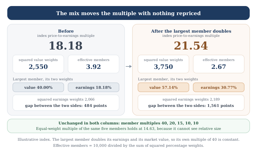
Market values across the five members now sum to 1,400 and earnings to 65. The index multiple is 1,400 over 65, or 21.54. It rose 3.36 points, or 18.5 percent, and not one of the five member multiples moved. The largest member's market-value weight went from 40.00 to 57.14 percent while its earnings weight went from 18.18 to 30.77 percent. The gap between those two shares is the entire effect.

Run the same exercise on the smallest member instead and the direction reverses. Double the member carrying 100 of market value and 10 of earnings, which trades at 10. Market values then sum to 1,100 against earnings of 65, for an index multiple of 16.92, or 1.26 points below where it started. The earnings-side statistic is identical in both experiments, because in each one a member's earnings of 10 became 20. The market-value side is not, and the next section measures it. What decides the sign is exact: doubling a member lifts the index multiple when its own multiple sits above the index multiple, and lowers it when it sits below.

The pair of experiments shows the channel rather than a direction. Mix alone moved the index multiple by 18.5 percent one way and 6.9 percent the other. It operates on something per-company valuation work does not price, because in this experiment the per-company answers never changed. Whether rising concentration lifts or lowers a multiple is a separate question, and it needs the statistic set out in the next section.

The equal-weight reading works as the control on both experiments. It holds at 14.63 in each, because none of the member multiples changed. The boundary on that control is that it only holds while nothing reprices.

Over a real period the members do reprice, and the two readings then diverge for two separate reasons. One is the mix of earnings weights. The other is that the two constructions put different weights on the same repriced multiples. Hold the earnings fixed instead and halve the largest member's price. Its own multiple drops to 20 while every earnings weight stays put. The capitalization-weighted multiple falls 20.0 percent to 14.55, and the equal-weight reading falls 6.8 percent to 13.64.

Measuring concentration: the sum of squared weights

The standard statistic for concentration is the sum of the squared member shares. The 2023 Merger Guidelines issued by the Department of Justice and the Federal Trade Commission define the Herfindahl-Hirschman Index that way. The document notes that it reaches 10,000 in a market served by one firm. It treats markets above 1,800 as highly concentrated, and an increase of more than 100 points as significant. Those shares are shares of a product market, and none of the antitrust thresholds transfer to an index. The numbers appear here because readers meet them in antitrust coverage, while the statistic itself carries over without any of that apparatus.

Summing the squares of the five market-value weights of the base index gives 2,550. After the largest member doubles it gives 3,750, a change of 1,200 points. The reciprocal is more readable: 10,000 divided by the statistic returns the effective number of members, meaning the count of equally weighted holdings that would produce the same figure. The base index of five names behaves like 3.92 equally weighted names, and afterwards like 2.67. A 500-name index sitting at 300 behaves like 33.3.

That statistic settles the direction question the last section left open. Doubling the smallest member takes the market-value side down to 2,355, and the effective count up to 4.25, so that case spread value out rather than concentrating it. To raise concentration and lower the multiple together, grow the same member sixfold instead. Market value then sums to 1,500 against earnings of 105, the multiple falls to 14.29, the statistic rises to 2,689 and the effective count falls to 3.72. Concentration therefore has no fixed sign. It lifts a multiple when weight gathers on members trading above the index, and lowers it when weight gathers below.

The refinement that matters for a multiple is to compute the statistic twice: once on market-value weights and once on earnings weights. Those are the two vectors the multiple actually uses. On the base index the market-value side reads 2,550 against an earnings side of 2,066, a gap of 484 points. After the largest member doubles, the market-value side reads 3,750 against an earnings side of 2,189, a gap of 1,561 points. The market-value side rose 1,200 points against 123 on the earnings side, so the gap between the two sides more than tripled. That divergence between the two sides is what moved the multiple from 18.18 to 21.54.

Two limits on the statistic are worth stating plainly before anyone leans on it. Index weights rest on float-adjusted share counts through the investable weight factor above, so this measures concentration of the investable float rather than of the underlying companies. And a squared-weight statistic describes weights only. It reports nothing about how the members' businesses relate to one another, so two indices at the same reading can hold very different sets of companies.

What concentration cannot tell you about index valuation

Three different composition problems get discussed under the same word, and they need separating. The pillar article on what CAPE measures treats composition drifting across decades, so a reading from one era does not compare cleanly with another. Sector multiples by industry treat dispersion across the members of one industry group, and why sector multiples differ treats the fundamentals behind those group figures. This article treats the weights inside one index at one moment. All three describe an aggregate that carries the weights used to build it, and none of them is a statement about a company.

What concentration will not do, at any reading, is settle a valuation. A high effective-number reading does not make an index cheap and a low one does not make it expensive, because the statistic contains no prices relative to fundamentals. It bounds how far an aggregate multiple can be read as describing a typical member, and nothing further. When the market-value and earnings weights of the top few members diverge widely, an index multiple has become a statement about those members. A mid-cap company compared against that aggregate is being measured against a handful of much larger ones.

Nor does concentration tell you which direction the aggregate will travel next. The statistic describes the current weights, and the sign of any future move depends on where the members gaining share happen to trade. That is a per-company fact, and no concentration reading contains it.

One omission here is deliberate: this piece quotes no current concentration reading. Any such figure dates within a quarter, and the current reading with its market interpretation sits in the US market valuation analysis. The arithmetic above holds at any level of concentration, and none of the worked figures depends on a current reading.

Where this sits in a company-level workflow

Concentration work belongs in the step where a benchmark gets chosen, not the step where a company gets valued. Before using any index or group multiple as a reference point, establish which weights built it. Then check whether the two weights of its largest members diverge, and what its effective number of members is. If a handful of names carry the figure, the aggregate is a description of those names. A narrower comparison group is the fix, and the effective-member count tells you when you need one.

The InvestViable Valuator runs a discounted cash flow from inputs the analyst sets: the cash flow growth path, the discount rate, and the terminal growth rate. No index-level statistic enters it. The InvestViable stock screener filters a universe of 3,000+ US stocks on fundamentals. Slices of the Stock Universe such as technology stocks narrow that universe to a single sector, one way to build the narrower comparison group. Reported earnings and share counts behind any weight calculation trace back to the filings themselves, searchable through SEC EDGAR.

The transmission from a market-level input to a company-level answer runs through the discount rate, not through the aggregate multiple. That path is the subject of how interest rates flow into stock valuation. Concentration is a property of the reference point rather than of the company, and establishing it costs one calculation on published weights. Skipping it leaves a bias in every comparison built on top of that reference.