How Interest Rates Flow Into Stock Valuation

The transmission chain, one step at a time

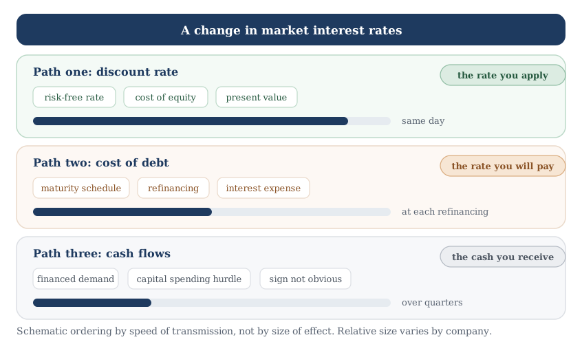
A rate change reaches a company's value along three separate paths, on different timescales.

The first path is the discount rate. By convention the risk-free rate underneath a cost of equity is a long government bond yield, usually the ten-year. That choice is about liquidity and habit, not about matching the duration of the cash flows. It carries a term premium and is not risk-free in real terms, but it is directly observable. The Federal Reserve publishes the 10-year Treasury constant maturity series daily. When that yield moves, the cost of equity moves with it, holding the equity risk premium and beta constant. It is the fastest of the three.

The second path is the cost of debt, and it splits in two. The rate that belongs in a weighted average cost of capital is the rate the company would borrow at today, so that leg reprices with the market immediately. The lag shows up in reported interest expense, which hits the cash flows in a free cash flow to equity model. In the firm model used here it does not, because the cost of debt sits in the discount rate and taxes are taken on unlevered earnings. Floating-rate revolvers and term loans reprice at once. Fixed-rate borrowings reprice only as they mature. A company refinancing a large tranche within two years feels a rate rise quickly, while one that termed out its borrowings for a decade barely feels it. The maturity schedule sits in the debt footnote of the annual report, available through SEC EDGAR. There is an offset on the other side. Existing fixed-rate debt at a below-market coupon becomes more valuable to the equity holder when rates rise, but only if you subtract debt at market value in the bridge. Subtract book value, as many models do, and that offset never reaches the answer.

The third path runs through the cash flows. Higher borrowing costs restrain customer purchases of financed goods, and they raise the hurdle a company applies to its own capital spending. The sign is not obvious. Cutting capital spending raises near-term free cash flow while lowering the growth the terminal value rests on, so this path can move the answer either way. It is also the slowest and the hardest to size.

Three different rates drive the three paths. The discount rate takes its anchor from the long end of the curve, floating-rate debt from the policy rate, and financed demand from short and mortgage rates. A curve that steepens can move the first path and leave the other two alone.

This article covers what happens when the rate environment changes. The discount rate and WACC walkthrough sets out that construction, from the cost of equity through to the after-tax cost of debt. Take it as given here. Everything below discounts free cash flow to the firm at a weighted average cost of capital.

Why distance multiplies a rate change

Present value divides a future cash flow by one plus the discount rate, raised to the number of years until it arrives. The exponent is what makes rates matter so much.

At an 8 percent rate, a dollar arriving in one year is worth about 93 cents. The same dollar arriving in ten years is worth about 46 cents, and in twenty years about 21.5 cents. Raise the rate to 9 percent and the one-year figure barely moves, falling to about 92 cents. The ten-year figure falls to about 42 cents, and the twenty-year figure to about 17.8 cents. The one-year figure lost about 1 percent of its value. The ten-year figure lost about 9 percent, and the twenty-year figure about 17 percent.

That asymmetry is the whole of the duration argument. Practitioners borrow the term from bond mathematics. There, duration is the average time until a bond's cash flows arrive, with each date weighted by that cash flow's share of present value. Divide that figure by one plus the yield and it gives the approximate percentage price move per point of yield change. Equity has no contractual maturity, so its duration has to be implied, and the transfer is only partial. A perpetuity-growth model implies an equity duration above eighteen years at the rates used below. Realized equity moves per point of yield have been smaller than that, because the premium and the growth outlook move at the same time. Treat duration as an ordering device for equities, and stop short of using it as a coefficient. A business whose cash flows arrive soon behaves like a short bond. A business whose value depends on what happens in year fifteen behaves like a long one.

Two things follow. First, a rate change lands unevenly across a portfolio, even when every holding is discounted at the same rate. Second, the sensitivity belongs to the forecast an analyst wrote, and a sector label will not settle it. A regulated utility funding a fifteen-year capital program carries more of its value in the far future than a profitable software business already returning cash.

The terminal value absorbs most of a rate change

Most of a growing company's present value sits in the terminal value, and that is the part a rate change hits hardest. The denominator is why.

A terminal value built on a perpetuity starts from the year after the final forecast year, which is the fifth-year cash flow grown once at the terminal rate. It divides that figure by the discount rate minus the terminal growth rate. That difference is usually small, so a change in the rate is a large proportional change in it.

Work it through on one set of numbers. A company generates 100 in free cash flow next year. That figure grows 6 percent a year from the second forecast year, so year five is 126.2. After year five it grows 2.5 percent forever. At an 8 percent discount rate the five explicit years are worth 446 and the terminal value is worth 1,601, for a total of 2,047. The terminal value is 78.2 percent of that total.

Now raise the discount rate to 9 percent, changing nothing else:

• Explicit five years: 446 falls to 434, a decline of 2.7 percent.
• Terminal value: 1,601 falls to 1,294, a decline of 19.2 percent.
• Total value: 2,047 falls to 1,728, a decline of 15.6 percent.

The terminal decline has two sources. The gap between the discount rate and terminal growth widens from 5.5 points to 6.5 points. Since 5.5 divided by 6.5 is 0.846, that accounts for a 15.4 percent fall on its own. The other 4.5 percent comes from discounting the same five years back at the higher rate. That drops the five-year discount factor from one over 1.08 to the fifth power to one over 1.09 to the fifth. The two effects multiply rather than add: compound 0.846 and 0.955 and the product is 0.808, the 19.2 percent decline.

That split is an artifact of the perpetuity convention. Build the terminal value from an exit multiple instead and the denominator term disappears: a multiple sets the terminal figure, and the rate no longer touches it. On the same numbers the terminal value moves only by that discount factor, and the one-point rise costs about 4 percent rather than 15.6. That insensitivity is bookkeeping, not economics. A multiple carries an implied rate inside it, and holding it fixed while raising the discount rate is the same inconsistency in another form. State which terminal convention you used; it is doing most of the work here.

That 15.6 percent holds the equity risk premium fixed and, as an enterprise value figure, excludes the market-value-of-debt offset. The limits section returns to both.

This is why terminal assumptions deserve the scrutiny the DCF inputs checklist gives them. A model whose terminal value carries four fifths of the answer is mostly an opinion about a denominator. The same arithmetic runs in reverse: a reverse DCF holds price fixed and solves for the implied growth, which the rate you fix decides.

Long-duration cash flows reprice hardest, and by how much

The duration argument above left an ordering as a prediction. With the terminal value now in place, that prediction can be tested. Each profile below starts from 100 in free cash flow next year, runs five explicit forecast years, and ends in a perpetuity. The ordering does hold, though the spread is narrower than the usual telling.

A flat business generating 100 a year is worth 1,250 at 8 percent and 1,111 at 9 percent. That is a fall of 11.1 percent. Split the same stream the way the other two profiles are split, into five explicit years and a perpetuity, and 68.1 percent of the value lands in the terminal. That share says very little about the business itself. The moderate grower from the previous section, with 78.2 percent of its value in the terminal, falls 15.6 percent. A faster grower, compounding 15 percent through the forecast years and 3 percent after, holds 82.3 percent of its value in the terminal and falls 17.3 percent.

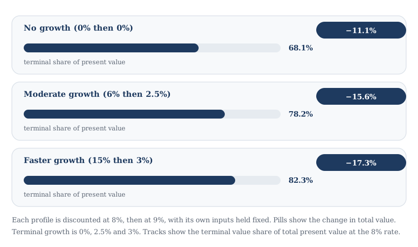
Six percentage points separate the least and most rate-sensitive profile here. The next section describes a modeling choice that can move a single valuation by fifteen points. These are different quantities, one cross-sectional and one inside one model, so read them as two separate reasons for care and resist ranking them.

Two cautions on reading that ordering. The first is that terminal share is a property of the forecast an analyst wrote. It describes the model more than the business. Push the explicit forecast out to ten years instead of five, holding the same cash flow path, and the terminal share falls without anything changing about the company. Compare terminal shares only across models built on the same horizon and the same conventions.

The second is that terminal share alone does not fix the sensitivity. Two profiles can carry almost the same terminal share and still reprice points apart. The terminal growth rate sets the denominator gap independently of the share. A flat stream with 3 percent terminal growth and a stream compounding 30 percent for five years into zero terminal growth both sit near a 78 percent terminal share. On the same one-point rise the first falls 16.5 percent and the second falls 12.4 percent. That pair is built to hold the share fixed, which is the point of it. The three profiles above vary explicit growth and terminal growth together, so read the ordering as illustrative and expect exceptions.

The inflation double-count

The duration effect above is arithmetic and unavoidable. What follows is neither, which is why it gets a section of its own. An analyst reads that rates have risen, raises the discount rate by a point, and leaves the growth assumptions exactly where they were. That produces the 15.6 percent decline computed above. It is often wrong.

A nominal discount rate contains an expected inflation component. So does nominal terminal growth, and so does the nominal cash flow forecast. If a rate rise is compensation for higher expected inflation, and the company can pass that inflation into its prices, then all three should move together. Even then the match is inexact. Depreciation tax shields sit on historic cost and do not inflate. Working capital investment scales with nominal revenue. A fully price-passing business therefore still leaks a little real cash flow to inflation. Removing inflation from one side of the model only is a units error, and it often gets defended as conservatism.

Run the consistent version. Raise the discount rate from 8 to 9 percent, raise terminal growth from 2.5 to 3.5 percent, and raise forecast cash flow growth from 6 to 7 percent. Total value goes from 2,047 to 2,045, a decline of 0.1 percent. That residual is the net of two small approximations. The first forecast year was left unescalated, and one point was added to each rate where compounding each by 1.01 would have been exact. Compound them exactly, at 7.06 percent, 9.08 percent and 3.525 percent on a first-year cash flow of 101, and the value comes back unchanged to the decimal. The real value of the business holds, which is the correct answer when nothing real has changed.

Note what that exactness rests on. The model above escalates a single free cash flow line, which carries no depreciation deduction. The historic-cost leak has nowhere to appear in it. Build the same case up from EBIT with an explicit depreciation schedule and the value does fall, by the present value of the tax shield the higher price level erodes. The zero here reflects the model's shape. It hides the leak rather than disproving it.

Read the rate move before reacting to it

A nominal yield has two legs, and which one moved decides whether any of the above applies. The Federal Reserve Bank of St. Louis publishes a 10-year breakeven inflation rate, the difference between the nominal and inflation-indexed Treasury yields. It gives a market-implied split of a nominal yield into an inflation piece and a real piece. That inflation piece also carries an inflation risk premium and a liquidity effect on the indexed leg, so treat it as a direction of travel.

A rise concentrated in the breakeven component is an inflation event. A rise concentrated in the real component asks a second question rather than settling it. If real rates rose because expected real growth rose, the same consistency test applies one level down. A higher real discount rate paired with an unchanged real growth assumption is not a units error. It is the same failure to update both sides of the model from one piece of news. Only a real-rate rise carrying no growth news with it compresses value cleanly. In practice both legs move together, so a rise driven purely by expected inflation is the special case and not the norm.

Full pass-through is an assumption to defend company by company. A business facing contractual pricing, regulated tariffs or intense substitution cannot raise prices with the index. For that business the value loss is real, and it belongs in the cash flow forecast where the pricing constraint actually lives, stated as an assumption a reader can check.

The same units error has a market-level version, in the spread quoted between an index earnings yield and a government bond yield. That comparison is the subject of earnings yield versus bond yield, and it is a separate question from the per-company transmission covered here.

What the mechanism does not tell you

The transmission is a sensitivity result. It says how much a value moves for a given change in the rate. Where rates go next, and whether any security is mispriced, are separate questions with separate evidence.

Five limits belong on the record.

The answer depends on conventions you chose. A perpetuity terminal value produces the denominator effect above and an exit multiple does not, so report which one you used alongside the number.

A one-point move in the market rate is not a one-point move in a weighted average cost of capital. The after-tax cost of debt rises by one point times one minus the tax rate, so a levered firm's blended rate rises by less. At 30 percent debt and a 21 percent tax rate the WACC rise is 0.94 points, and the decline is 14.8 percent instead of 15.6.

The headline number holds the equity risk premium fixed, and the premium does not hold fixed. Damodaran publishes an implied equity risk premium series rebuilt each year from index prices and expected cash flows, and it moves in both directions against yields. It compressed as the ten-year rose through 1999, and again through 2024. It expanded from 4.24 to 5.94 percent while the ten-year went from 1.51 to 3.88 percent across 2022. Read 15.6 percent as the arithmetic with one input frozen, not as a bound in either direction.

You have today's rate, and today's rate is the only one you have. Building a valuation on a projected rate path swaps an observable number for a guess, and the guess inherits every weakness of macro forecasting. Read the current rate from a primary release such as the Federal Reserve's H.15 selected interest rates, record the date, and rerun later.

A sensitivity result says nothing about whether a price is right. A model showing that value falls 15.6 percent on a one-point rate rise has established a property of that model. The market may have repriced already, or may be pricing a different premium than the model assumes.

The repricing itself is capital-market news, so it belongs in the rate. Resist taking a second haircut to the cash flows for the same repricing, and resist widening the margin of safety for it on top of that. Demand and pricing effects are a separate mechanism, and they belong in the forecast only where you can name the constraint and defend it. That stacking problem is set out in full in the discount rate and WACC walkthrough.

The market-level version of the same caveat sits in the pillar article on what CAPE measures and where it fails. That piece notes a high reading does not account for prevailing rates. Neither converts a rate observation into a timing signal, and neither is trying to.

How to apply this

Start by writing down the rate you used and the date you read it, because an undated discount rate cannot be checked by anyone, including you six months later. Then run the valuation across a band of rates. A one-point range on either side is a reasonable default, and the sensitivity analysis method covers how to present the output as a range. Record what share of your value sits in the terminal value, alongside the horizon that produced it. That share is comparable only within one set of conventions. The moderate profile above sits at 78 percent on five explicit years and 60 percent on ten. The cash flow path and the total value of 2,047 are identical in both. Keep the units consistent, so a nominal rate meets nominal growth.

The InvestViable Valuator runs a discounted cash flow from user-set inputs. It takes the cash flow growth path, the expected return you demand as the discount rate, and the terminal growth rate. Run it at each end of your rate band and read the two values as a range.

A rate is an input you share with every other holder of every other stock. Nobody is working from a number the market has not already seen, so on its own it cannot tell you which stock is mispriced, however unevenly it lands across them. The InvestViable stock screener filters a universe of 3,000+ US stocks on fundamentals. Sliced views such as the growth-style slice of the Stock Universe apply thresholds to those same fields.