
Sector multiples differ because the businesses inside them convert profit into distributable cash at different rates and carry different risk. A justified price-to-earnings multiple equals the payout ratio times one plus growth, divided by the cost of equity minus growth. Payout is whatever survives retention, and retention equals growth divided by return on equity. A sector earning 25 percent on equity funds 5 percent growth by retaining 20 percent of its profit, while one earning 8 percent must retain 62.5 percent. Hold growth and the cost of equity identical across both, and the first still justifies roughly twice the multiple of the second.
What a sector multiple is made of
A multiple looks like a shortcut around a discounted cash flow model, and rearranging that model's terms produces it exactly.
Take a company growing at a constant rate forever. Under the Gordon growth model its value equals next year's dividend divided by the cost of equity minus the growth rate. Divide both sides by current earnings and the trailing price-to-earnings multiple falls out: payout ratio times one plus growth, over the cost of equity minus growth. Published sector multiples come in both bases; the forward version drops the one-plus-growth term from the numerator, so match the basis before you compare. The discounted cash flow method is still doing the work underneath.
What the payout ratio hides matters more than the rearrangement. A company cannot pay out what it needs to retain, and what it retains depends on how efficiently it converts equity into profit. The sustainable growth identity ties the two together. Growth equals the retention rate times return on equity, so retention equals growth divided by that return, and payout is one minus retention. The multiple reduces to three primitives: return on equity, the growth that return can sustain, and the cost of equity.
Every sector-level difference in multiples enters through one of those three. Everything else is measurement error: an earnings figure that fails the formula's assumptions, a metric that excludes reinvestment altogether, or an aggregate whose weights belong to somebody else. Those three failures are the second half of this article.
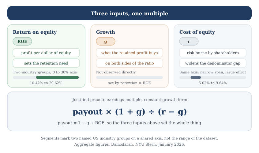
Figure 1. Three inputs, one multiple
Payout is not independent: it is what remains after retention, and retention is growth divided by return on equity. The spans mark general utilities against system and application software.
One bookkeeping rule keeps this usable: return on equity, payout and the cost of equity are equity-side quantities, and they belong with a price-to-earnings multiple. The firm-side version of the same algebra uses return on invested capital, a weighted average cost of capital and an enterprise value multiple. That is where the EBITDA section below operates.
That framework drains the phrase "trading above its sector" of most of its content. Two businesses with different returns on equity should trade at different multiples, and a gap between them that traces to one of the three primitives is explained. The gap that deserves attention is the one none of the three accounts for.
Which valuation route suits a given business is a separate question, covered in choosing a valuation method. This article assumes you have already decided to look at a multiple.
Return on equity sets the price of growth
Growth is not free, and return on equity sets its price. Holding growth and risk fixed, this is what separates two sectors' multiples.
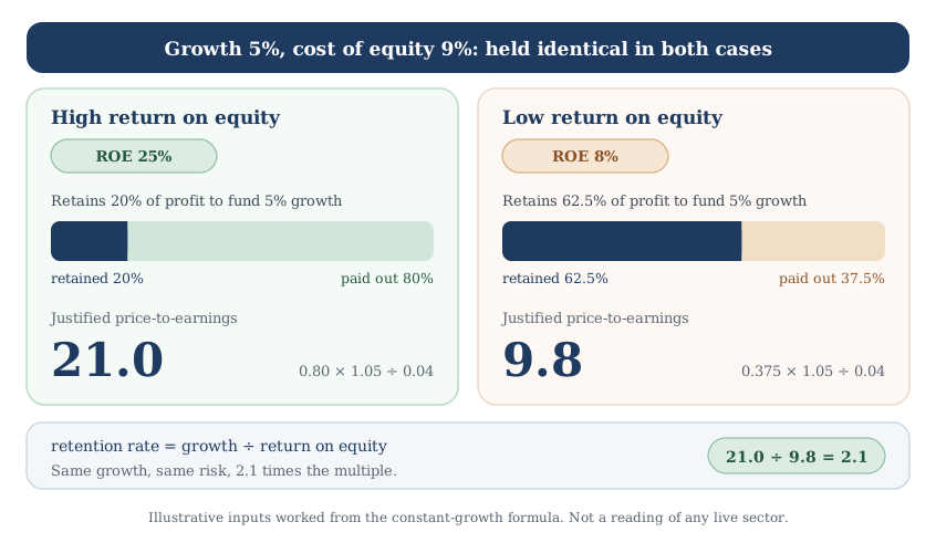
Take two sectors that both grow earnings at 5 percent a year and both face a 9 percent cost of equity. The first earns 25 percent on equity, so it funds that growth by retaining 5 divided by 25, or 20 percent of profit, and pays out 80 percent. Its justified multiple is 0.80 times 1.05, divided by 0.04, which is 21.0. The second earns 8 percent, so it must retain 5 divided by 8, or 62.5 percent, and pays out 37.5 percent. Its multiple is 0.375 times 1.05, divided by 0.04, which is 9.8.
Growth and risk are identical across the two, and the first justifies a multiple 2.1 times as high, produced entirely by the efficiency of the reinvestment. An investor calling the second sector cheap on that comparison would be reading the cost of its growth as a discount.
Figure 2. Same growth, same cost of equity, different return on equity
Both sectors grow at 5 percent and are discounted at 9 percent. The only difference is how much profit each must retain to fund that growth.
The dispersion in real data is wide enough to change the answer. In Damodaran's January 2026 US dataset, aggregate return on equity is 10.42 percent for general utilities and 29.62 percent for system and application software. The market excluding financials sits at 17.60 percent, and basic chemicals sit at negative 8.29 percent. Those groupings are Damodaran's own industries, not GICS. Roll them up into the eleven GICS sectors and the spread between sector averages narrows, while the spread hidden inside each one gets wider.
The inference does not run backwards: a high retention rate implies nothing about the level of the return, since growth equals retention times return on equity. A fast-growing high-return business retains heavily too. Which version of the return belongs in a given calculation is settled by the difference between return on invested capital, return on equity and return on assets.
The discount rate can outweigh the return
Risk enters through a denominator, which makes it stronger than its size suggests.
Hold the fundamentals fixed and vary only the cost of equity. A sector earning 15 percent on equity, growing at 4 percent, retains 26.7 percent of profit and pays out 73.3 percent. At an 8 percent cost of equity the justified multiple is 19.1. At 10 percent it is 12.7. Two points on the cost of equity cost a third of the multiple. The rate sits in a denominator alongside growth, so the gap between them widens proportionally faster than the rate moves.
Observed spreads across industry groups run wider than two points. The same dataset puts aggregate cost of equity at 5.02 percent for general utilities and 9.64 percent for system and application software. Regulated revenue and long contracted asset lives hold the first down; uncertain terminal outcomes and high operating leverage push the second up.
Now set the two inputs against each other, using those two real groups. Impose 2 percent growth on both, as a test of the algebra rather than a description of either business. The formula returns 27.3 for the utility group and 12.4 for the software group, and the higher-return group is the one that loses. Software's advantage on return surfaces only as a lighter retention burden: the model implies it pays out 93.2 percent of profit against the utility's 80.8 percent. That margin cannot overcome a denominator more than two and a half times as wide, at 7.64 points for software against 3.02 for the utility.
Which of the two effects wins is decided by the growth rate, and growth is bounded by the return that funds it. It equals retention times return on equity, so the return is its ceiling. Give both groups a 40 percent retention rate. Implied growth reaches 4.2 percent for the utility and 11.8 percent for the software group, above its own 9.64 percent cost of equity. The expression then returns a negative number, which is worse than no answer because it still looks like one. Businesses that grow fast on high returns get modeled in stages for that reason. The single-stage form used here decomposes a multiple; it does not compute one for a whole sector.
Constructing the discount rate is its own exercise, set out in the discount rate and WACC walkthrough. The market-wide version of the same question, what return investors demand in aggregate, sits in earnings yield against bond yield. One narrower point belongs here. A sector-level cost of equity is an average of company-level costs, and leverage varies inside a sector, so a levered cost of equity moves with it.
What EBITDA leaves out
Enterprise value to EBITDA is the multiple most exposed to the reinvestment problem, because EBITDA is defined by what it excludes. This section runs firm-side, so the return concept is return on invested capital and the discount rate is a weighted average cost of capital.
Set two companies side by side, each reporting EBITDA of 100. The first carries depreciation of 10 and spends 12 on capital. Its operating income is 90, and its after-tax operating income at a 21 percent rate is 71.1. Free cash flow to the firm is 71.1 plus 10 minus 12, or 69.1, before working capital, which is held at zero throughout. The second carries depreciation of 35 and spends 40. Its operating income is 65, after-tax operating income is 51.35, and free cash flow is 46.4. Same EBITDA, and 49 percent more cash from the first.
Discount both at the same 6 percent spread between discount rate and growth, held identical so that only the cash flows differ. The enterprise values come out at 1,152 and 773. Treating current free cash flow as the perpetuity numerator understates both by one year of growth and leaves the ratio between them unchanged. The implied EV/EBITDA is 11.5 against 7.7, from identical EBITDA. Apply the first company's multiple to the second and you overprice it by about half; apply the second's to the first and you underprice by about a third.
Capital intensity of that kind travels with the business type rather than the individual company. In Damodaran's January 2026 capital expenditure dataset, capital spending runs at 315.04 percent of depreciation for general utilities and 80.48 percent for pharmaceuticals. Net capital expenditure consumes 166.93 percent of after-tax operating income in general utilities, against 40.90 percent across the market excluding financials. A utility replacing and expanding the regulated asset base it earns a return on has a structurally different claim on its own EBITDA. A business whose depreciation exceeds its capital spending does not face the same call on cash.
EV/EBITDA therefore compares businesses correctly only when their reinvestment profiles are similar, which is what a sub-industry grouping is supposed to deliver. The mechanics of the EBITDA multiple cover the enterprise-value bridge in full, and the gap between headline profit and cash is the subject of owner earnings versus free cash flow.
What sector multiples average away
Everything above treats a sector as though it had one set of fundamentals, and no sector does. A sector figure is a summary statistic, and how it gets computed determines what it can support.
Damodaran's industry tables aggregate dollars across constituents and then divide. The capital expenditure table reports total capital spending and total depreciation for each industry before showing the ratio between them. Dollar weighting hands the number to the largest contributors to the denominator. Index-level sector multiples use a different weight, float-adjusted market capitalization under a published float adjustment methodology, which concentrates the figure on the same large constituents for a different reason.
Loss-making constituents distort the same aggregates from the other direction. A multiple computed across all firms in a group carries companies with negative or near-zero earnings in its denominator, which lifts the group figure. The same group measured across profitable firms gives a lower multiple, so state which basis you are using.
Classification adds a second layer on top of the weighting. Under the Global Industry Classification Standard, each company receives a single classification at each of four tiers. The assignment follows principal business activity, with revenue as the key factor, though earnings and market perception are also weighed at the annual review. A company with three businesses still lands in one bucket.
The pillar article on what CAPE measures treats the same problem across time instead of across members. There, the composition of an index shifts over decades, so a reading from one era does not compare cleanly with another. Here the composition varies across the members of one group at a single moment, and in both cases the aggregate carries the weights used to build it.
Current levels for the major sector multiples, and the forces moving them, are the subject of the sector multiples benchmarking guide. This article stays on the mechanism, which does not change when the levels do.
What the earnings figure fails to measure
A sector's multiple can also look strange because the earnings figure underneath it fails to measure what the formula assumes.
Cyclical sectors are the clearest case, because the constant-growth formula wants a sustainable earnings level and a commodity producer at a cycle peak reports something else. Its multiple compresses precisely when its earnings are least repeatable, which inverts the signal for anyone reading the multiple alone. Running the earnings normalization for cyclical businesses first does the work the multiple cannot do for itself.
Financials break the enterprise-value family from the other end, where the problem sits in the numerator. Debt is raw material for a bank rather than financing, so subtracting cash and adding debt produces a figure with no economic meaning. Equity-side metrics such as price to book, read against return on equity, hold up where enterprise-value metrics do not.
Accounting treatment supplies the last case, and it runs deepest. Most research and development is expensed as incurred, so the asset it builds never appears in book equity or invested capital. Research-heavy sectors therefore report understated capital and, where research spending is stable, overstated returns on it. Software is a partial exception, since some development costs are capitalized once a project passes a defined stage, though the capitalized share is usually small next to total engineering spend. The distortion is systematic by sector, which embeds it in every sector average built from reported figures.
Reading the gap between your multiple and the sector's
Build the multiple your own inputs imply, set it beside the one the market quotes, and treat the difference as a question.
Say your estimates give a company a justified multiple of 14 and its sector trades at 20. Three explanations compete. Your inputs may be wrong, most often the return on equity or the sustainable growth rate. The market may be assuming something you have not, in which case a reverse discounted cash flow extracts the assumption and lets you argue with it explicitly. Or the company may genuinely differ from its group on one of the three primitives, which counts as a finding.
Only the third is a valuation conclusion, and it still needs a range around it. The width of that range comes from testing which inputs the answer depends on, which is what a sensitivity analysis is for. Single-point estimates produce a justified multiple carrying more apparent precision than the inputs support. Rank the three primitives by how far each would have to move to close the gap on its own. That ranking tells you which one to check first.
Work through the first explanation before reaching for the third. Your own estimate is the cheapest to test, since you already hold every input that produced it. An error there is also more common than a mispriced sector.
The order matters for a reason that is easy to miss. Reverse-engineer fundamentals from the sector multiple first, and whatever you build agrees with the market by construction.
Where sector valuation fits in a company decision
Sector valuation is a diagnostic layer, and it values nothing itself. The step that decides everything downstream comes first: identify the narrowest grouping whose economics your company actually shares. A GICS sub-industry narrows the group, and a hand-picked set of genuine peers narrows it further at the cost of a smaller sample. Estimate that group's return on equity, sustainable growth and cost of equity from its own reported figures instead of from its quoted multiple.
The InvestViable Valuator runs a discounted cash flow from inputs you set: the cash flow growth path, the discount rate, and the terminal growth rate. Sector work belongs upstream of it, in deciding what those inputs should be for a business of this type. The InvestViable stock screener filters a universe of 3,000+ US stocks on fundamentals. Sector slices of the Stock Universe such as energy, technology and utilities apply the same fields inside one grouping. Reported earnings, book equity, capital spending and depreciation all trace back to the filings themselves, searchable through SEC EDGAR.
One habit pays for itself. Whenever a sector average enters your analysis, write down which of the three primitives you are borrowing from it and which you are estimating yourself. The common failure is borrowing all three by accident.
InvestViable does not publish buy or sell recommendations on individual securities. All analysis is based on public financial data and a transparent methodology. The Investment Score formula is proprietary; the inputs and what the score evaluates are documented.