Cost of Equity: A CAPM Beta You Can Defend

What the number is, and what it is not for

The capital asset pricing model, or CAPM, sets the cost of equity as the risk-free rate plus beta times the equity risk premium. Two of those three inputs are shared across every company in a market. The discount rate and WACC walkthrough covers how the whole rate is assembled, and the piece on which equity risk premium to use covers the premium. Beta is the only term specific to one business.

Systematic risk only, in other words, scaled to a market of 1.0. A business can be volatile on its own and still add little to a diversified holding. A reading of 1.4 says nothing about a company's risk in isolation.

Worry about a company's accounting quality, its customer concentration or its succession risk belongs in the cash flow scenarios, where a diversified holder has not already diluted it. Loading those into beta risks charging for the same risk twice.

One convention decides whether any of the arithmetic below applies to your model. A cost of equity discounts cash flow to equity holders. Firm-level cash flow is discounted at the weighted average cost of capital instead, and mixing the two credits the company twice for cheap debt. Every figure computed in this article is equity-side.

The three choices that produce the number

Damodaran's paper on estimating risk parameters works one company through each choice. The figures below are for Disney on monthly data from January 1993 to December 1997, except where the choice under test varies. They are dated illustrations rather than current readings, nothing below is a valuation of that company, and the cash flow stream used to price the estimates is invented. This is a test of the arithmetic.

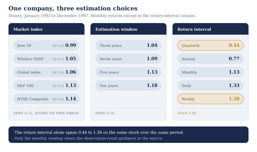
Index first. Against the Dow 30 the beta came out at 0.99. Against the S&P 500 it was 1.13, the NYSE Composite 1.14, the Wilshire 5000 1.05, and a global equity index 1.06. That is a span of 0.15 on one stock. No index is the market portfolio the model assumes, so the answer moves with the subset you pick. Read the span against the standard errors the same table reports, which run from 0.18 to 0.24: the five estimates are statistically indistinguishable from each other.

Window next. Over three years the beta was 1.04, over five 1.13, over seven 1.09, over ten 1.18, a span of 0.14. Longer windows buy more observations, and they reach back to a period when the company carried a different business mix or debt load.

The return interval moves it most. Daily returns produced 1.33, weekly 1.38, monthly 1.13, quarterly 0.44 and annual 0.77. Only one of those five earns the source's endorsement. Over a five-year window, quarterly gives about twenty observations and annual gives five, too few to read; daily and weekly carry a non-trading bias covered later. Damodaran's guidance is monthly for a firm listed more than three years.

Taking the extremes across the index and window columns, 0.99 and 1.18, gives a pair worth pricing. Use the 10-year Treasury yield of 4.73 percent recorded on August 28, 2026 in the Federal Reserve series and Damodaran's implied equity risk premium of 4.23 percent entering 2026. Those two carry different vintages, a mismatch worth naming and then holding constant. What a moving rate environment does to the rest of the model is covered separately. A beta of 0.99 gives a cost of equity of 8.92 percent; 1.18 gives 9.72 percent. Discount 100 of next-year cash flow, growing at 2.5 percent in perpetuity, at each rate. The values are about 1,558 and 1,385. Two estimates a statistician cannot separate still price 12.5 percent apart.

The confidence interval that rarely travels with the number

A regression beta is a point estimate with a standard error attached, and the standard error almost never travels with it.

Damodaran reports both for the same company. Against the S&P 500 the beta was 1.13 with a standard error of 0.22. At 67 percent confidence the true beta sits between 0.91 and 1.35, and at 95 percent he puts the range at 0.69 to 1.57.

Pushed through the same build-up, that wider range gives costs of equity from 7.65 to 11.37 percent. On the same perpetuity the values are about 1,942 and 1,127. The top sits 72 percent above the bottom, and every point inside is consistent with the regression that produced the headline 1.13. Part of that gap belongs to the growth assumption: set terminal growth to zero and it narrows to about 49 percent, which is still most of the answer.

Damodaran also charts standard errors across all US stocks, and notes how many carry errors above 0.50. He describes those as close to useless by themselves, so Disney is not an unusual case. A beta of 1.20 with a standard error of 0.55 cannot separate a defensive business from an aggressive one.

Arguing over whether a beta is 1.15 or 1.20 is therefore arguing inside the noise, and a valuation that turns on the distinction is unsupported by its own input. The practical consequence is a habit: whenever you take a beta from any source, ask what its standard error was. If the source publishes none, treat the figure as approximate and widen accordingly. The sensitivity analysis method covers how to present the result.

Why data services shrink beta toward one

Many data services do not report the raw regression slope. They report an adjusted beta, pulled toward 1.0 by a fixed formula that weights the regression estimate 0.67 and the market average 0.33.

Applied to the Disney estimates, the weekly 1.38 comes back as 1.25, the daily 1.33 as 1.22, the monthly 1.13 as 1.09 and the quarterly 0.44 as 0.62. Every reading is compressed toward the middle, and the low ones move hardest in proportional terms.

The rationale the services give for this is sound. Companies that survive tend to grow and diversify, which pushes a beta toward the market average over time, and an estimate of next decade's risk should reflect that drift. Damodaran's objection lands on the fixed weights. The same 0.67 is applied whether the standard error is 0.10 or 0.60, though the second case deserves far more shrinkage. His own prescription is not a better formula. He argues against adjusting a regression beta at the estimation stage at all, and for letting it move toward one across the forecast periods themselves.

What matters in practice is narrower than the debate. Know which one you have. An adjusted beta and a raw beta are different quantities, and a model that mixes them across companies compares its own inputs. If your source publishes both, pick one convention and hold it for the whole exercise. If it publishes only the adjusted figure without saying so, the number in your model has already been moved a third of the way toward 1.0 before you saw it.

When a regression beta means nothing at all

Some regressions produce a number that looks fine and describes nothing. Four situations account for most of them.

• Thin trading. When a stock does not trade in many of the return periods, its measured correlation with the index falls and the beta comes back too low. In practice the diagnostic that discriminates is the count of zero-return periods inside the window. R-squared does not, since it runs low on single-stock regressions as a rule. Longer return intervals reduce the bias and cost observations.
• A short listing history. Damodaran puts the threshold at roughly three years of listing before monthly returns give enough observations to be worth reading. A company public for eighteen months sits inside that threshold on any interval, and no choice of window repairs it.
• Structural change. A regression run over five years describes the company's average business mix and average leverage across those five years. If it sold a division, made a large acquisition or repaid most of its debt inside the window, the beta describes a business that no longer exists. Shortening the window widens the standard error; keeping it leaves the estimate stale. Nothing in the output flags either, which is what makes this one easy to miss.
• Index domination. Damodaran's example is Telebras, which made up 40 percent or more of the Brazilian Bovespa index. Every other stock in that market was effectively being regressed against that one company. The largest and most established firms carried the highest betas, and the smallest and riskiest carried the lowest, which inverts the ordering the model expects. This is one reason ADRs and foreign-listed shares need care over which index the risk is measured against.

In all four the repair is the same, and it is not a better regression. The estimate has to be assembled from the businesses the company is in.

Bottom-up beta: assembling one from the industry mix

The alternative drops the company's own price history. A bottom-up beta is built from the businesses it operates in, then adjusted for how much debt it carries.

Five steps produce one. Identify the businesses the company is actually in. Take an unlevered beta for each from the industry averages. Weight them by the value of each business, using revenue or operating income when segment market values are unavailable. Establish the current debt-to-equity ratio and tax rate. Relever the weighted unlevered beta at that structure.

What makes this better is statistical rather than conceptual. Individual regression betas are noisy, but averaging across many of them cancels much of the noise. The standard error of an average falls with the square root of the number of firms. On Damodaran's illustration, an average standard error of 0.50 across 225 software firms gives a standard error on the average of about 0.03. His industry beta dataset covers 309 firms in the dataset's Software (System & Application) row as of January 2026, which on the same assumption gives essentially the same figure. The square-root rule assumes the individual errors are independent. Betas regressed against the same index over overlapping periods are not, so read the result as a floor on precision.

Two further properties come free with it. A bottom-up beta describes the business mix the company has today. It is also available for companies a regression cannot reach, including recent listings and divisions valued separately.

The same dataset shows how much the underlying business matters. Across the industries covered in January 2026 the levered betas run from 0.24 for general utilities to 1.69 for internet software, on 14 and 29 firms. At the risk-free rate and premium used above, that is a cost of equity spanning 5.75 to 11.88 percent. The gap is more than six percentage points before any company-level adjustment. Those endpoints also carry very different capital structures, at 81 and 12 percent debt to equity. Strip the leverage out and the underlying business risk still runs from 0.15 to 1.55. Those are the dataset's own unlevered figures, stripped at each industry's effective tax rate rather than a marginal one. The Stock Universe pages group coverage on the standard sector classification, which is broader than these industry definitions and averages much of that spread away, including utilities and technology.

Relevering: what capital structure does to the same business

Financial leverage raises the beta of a company's equity without changing the risk of its underlying business. Fixed obligations to lenders amplify what reaches shareholders in both directions.

The relevering identity states it directly: βL = βU × [1 + (1 − t) × D/E]. A levered beta is the unlevered beta multiplied by one plus the after-tax debt-to-equity ratio. The tax term appears because interest is deductible, which softens the amplification.

That form assumes the debt itself carries no market risk, which is where the identity is weakest at exactly the leverage that matters. Damodaran names the assumption and gives a corrected version, βL = βU × [1 + (1 − t) × D/E] − βD × (1 − t) × D/E. The subtracted term is the slice of market risk the lenders carry instead of the shareholders. Debt does bear that risk at high debt ratios, so the simple form overstates the levered beta there. At a debt beta of 0.10 the 75 percent case below falls from 1.96 to 1.90, and its cost of equity from 13.02 to 12.77 percent. The simple form is used below because it is the one in general use, and a reader working at high leverage should carry the correction.

Work the identity on one business. Use the unlevered beta of 1.23 that Damodaran's January 2026 dataset reports for system and application software, with a 21 percent marginal tax rate. That published figure was unlevered at the dataset's own effective rate of 5.51 percent, so relevering at 21 percent is an approximation. The three capital structures below are invented.

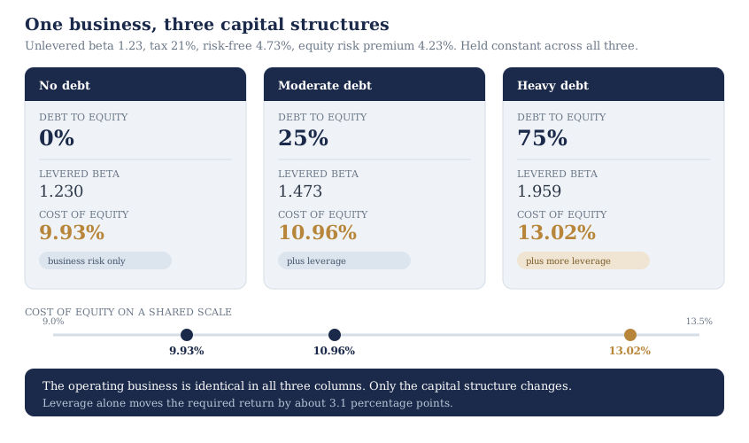
With no debt the levered beta stays at 1.23 and the cost of equity is 9.93 percent. At a debt-to-equity ratio of 25 percent it becomes 1.47 and 10.96 percent. At 75 percent, 1.96 and 13.02 percent. The operating business is identical in all three columns, and capital structure alone moves the required return by about 3.1 percentage points. Resist reading that as a value comparison: leverage also shrinks the equity cash flow being discounted, so holding the numerator fixed across the three columns would invert the result.

Whether the relevering is right comes down to three details. Use market values for both debt and equity, since the model prices claims and not historical cost. Use a marginal tax rate; a trailing effective rate carries one-off items that will not repeat. When leverage changed recently, unlever the old regression beta at the average ratio over the window before relevering at today's. Current debt balances and interest terms are in the latest 10-K on SEC EDGAR.

Record the five inputs, then report two numbers

Pick the construction before you pick the number, then hold it across the whole exercise. A bottom-up beta relevered at current market-value leverage is the default that survives the most scrutiny. It is also available for companies whose price history cannot support a regression at all.

Record five things beside the beta:

• the industries and their weights
• the unlevered betas, and the vintage of the dataset they came from
• the debt-to-equity ratio and its measurement date
• the tax rate, and whether it is marginal or effective
• whether any regression input was raw or adjusted

A cost of equity of 9.9 percent tells a reader nothing on its own. The same figure with those five lines beneath it can be checked and rerun six months later, which is what auditing a set of DCF inputs actually requires.

Then run the valuation at both ends of a beta band you can defend and present two values. The standard error on a single-stock regression is wide, and the industry vintage ages as you use it. The model itself is contested too. Fama and French, reviewing it in the Journal of Economic Perspectives, found its empirical record poor enough to invalidate the way it is used in applications. It remains the standard build because the alternatives are harder to source.

The band is easiest to run in a tool that exposes the rate directly. The InvestViable Valuator runs a discounted cash flow from user-set inputs. It takes the cash flow growth path, the expected return you require as the discount rate, and the terminal growth rate. Run it once at each end of your band and compare the two outputs. The tool takes the rate you set and does not derive it. Running several methods to one range shows how a cost of equity sits alongside other methods, and the pillar guide to valuation methods covers the surrounding workflow. Company selection is a separate step, and the InvestViable stock screener covers a universe of 3,000+ US stocks on fundamentals and the Investment Score.

Averaging your way to a single point discards the one thing the estimate reliably tells you, which is how uncertain it is.