Multi-Method Stock Valuation: Three Models, One Range

What a multi-method stock valuation produces

The habit of running several methods is easy to state and rarely worked through end to end. Execution raises questions that only appear once real numbers are on the page. Which earnings figure does each method get? And what do you report when three defensible calculations return three different answers?

This article answers those questions by performing the exercise. The valuation methods guide covers what each method is. Choosing which valuation method to use covers picking the right one for a given business. Why valuation methods disagree covers the structural reasons the outputs diverge. What follows is the arithmetic those three articles describe, run once, on one company, with every input sourced.

The company is Colgate-Palmolive. It satisfies each method's entry condition. The discounted cash flow model needs positive free cash flow. The earnings multiple and the Graham formula need positive reported earnings in the filed year. It also has a defined peer industry in the reference dataset and single-digit revenue growth over 2021 to 2025. Where a method fails on inputs like these, the structure of the method is what failed.

One framing note before any number appears. This tests the algebra. It does not describe the business. The point is to show what each method does with an identical set of filed inputs, and where the outputs part company. No figure below is a view on the security.

Every figure comes from the company's filings on SEC EDGAR, from the Federal Reserve Bank of St. Louis, or from Aswath Damodaran's published datasets. Market-dependent inputs are dated where they are used.

Normalize first, because the methods do not see the same year

The filed 2025 income statement includes a 582 million dollar goodwill impairment. Reported diluted earnings per share came in at 2.63 dollars, down from 3.51 dollars in 2024. Operating cash flow moved the other way, reaching 4,198 million dollars against 4,107 million a year earlier.

A non-cash charge cut the earnings figure and left the cash figure untouched. Any earnings-based method now reads a worse year than any cash-based method does, before a single modeling choice has been made. Normalizing is what stops that accident from being mistaken for information.

The add-back is 582 million dollars across 811.1 million diluted shares, or about 0.72 dollars per share. Normalized net income becomes 2,714 million dollars and normalized diluted earnings per share becomes 3.35 dollars. The charge is added back without a tax adjustment, on the basis that goodwill impairment is commonly non-deductible. If part of it were deductible, the add-back would be smaller and every earnings-based figure below would fall slightly. Normalized earnings still sit below the 3.51 dollars of 2024, so the impairment is not the whole of the decline. The DCF inputs checklist covers verifying each input before any method consumes it.

One check ties the reported figures together, and one derivation produces the cash input. Reported net income of 2,132 million over 811.1 million diluted shares returns 2.6285 dollars, which is the filed 2.63 dollars. Free cash flow, taken as operating cash flow less the 564 million dollars of capital expenditure, is 3,634 million dollars, or 4.48 dollars per share.

Two qualifications attach to that 4.48 dollar figure. Cash per share exceeds normalized earnings per share by 1.13 dollars, about 920 million. The impairment does not explain that gap, because it has already been added back on the earnings side. The difference is depreciation, amortization and other non-cash items plus working-capital movements, net of the 564 million dollars of capital spending. Second, operating cash flow is consolidated while the 811.1 million diluted share count is not. Consolidated FY2025 net income was 2,261 million dollars against 2,132 million attributable to Colgate-Palmolive. About 5.7 percent of this stream therefore belongs to noncontrolling interests, and the 4.48 dollar figure is an upper bound. The two earnings-based methods below do not carry that overstatement. Normalizing earnings covers the wider set of adjustments this step can involve.

Normalized earnings per share of 3.35 dollars and free cash flow of 3,634 million dollars now feed all three methods. Nothing downstream is allowed to use a different figure.

Method one: discounted cash flow from three inputs

State the convention before the arithmetic, because the convention moves the answer. This model discounts free cash flow to equity, defined as operating cash flow less capital expenditure, at the cost of equity. Net borrowing is set to zero. That is a simplification, not part of the definition. Held to perpetuity it implies leverage declining toward zero, so the constant discount rate below is an approximation. Operating cash flow is already net of interest paid, so the stream belongs to shareholders. The result is an equity value directly. Net debt is not subtracted; subtracting it would double-count the debt service already inside operating cash flow.

The cost of equity is built up from observable inputs. The 10-year Treasury yield stood at 4.64 percent on August 25, 2026, per the Federal Reserve series. Damodaran's implied equity risk premium series puts the premium at 4.23 percent on a free-cash-flow-to-equity basis at the end of 2025. His industry beta dataset gives Household Products a levered beta of 0.82 across 110 firms, as of January 2026. That gives 4.64 plus 0.82 times 4.23, or 8.11 percent. Two limitations belong with it. The premium and the risk-free rate are dated differently. And the 0.82 is a bottom-up industry average, levered at the industry's average debt-to-equity ratio. Used directly it prices the industry's leverage, not the company's. Relevering to the company's own capital structure is a step not performed here.

Growth comes from the filings. Revenue compounded at 4.0 percent between 2021 and 2025, rising from 17,421 million dollars to 20,382 million. The explicit period runs five years at that 4.0 percent rate. Applying a revenue growth rate to a cash-flow stream assumes margins and capital intensity hold. Terminal growth is set at 2.5 percent, well below the 4.64 percent risk-free rate.

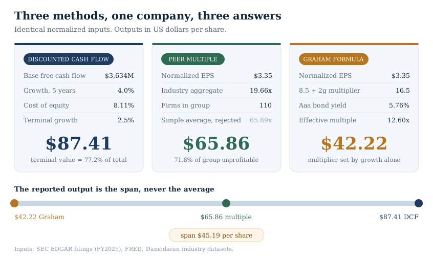
Discounting the five explicit years and a perpetuity-growth terminal value at 8.11 percent returns an equity value of 70,899 million dollars, or 87.41 dollars per share.

What the discounted cash flow figure depends on

The terminal value supplies 77.2 percent of that number. A five-year explicit period at an 8.11 percent discount rate and 2.5 percent terminal growth produces exactly that. The perpetuity-growth convention is itself a choice, and naming it matters because the alternative lands somewhere else.

Replacing it with the peer aggregate of 19.66 times, applied to year-five normalized earnings, returns 74.17 dollars per share, 15.2 percent below the perpetuity-growth figure. That is not a pure change of convention. It imports Method Two's peer pricing into the terminal value, which is most of the reason the two outputs move toward each other.

The sensitivity is wide enough to report. Hold growth at 4.0 percent and move the cost of equity from 7.11 to 10.11 percent. With terminal growth between 1.5 and 3.0 percent, the per-share figure runs from 58.64 to 117.42 dollars. Those are opposite corners of the grid, not a one-variable sweep.

Method two: what the peer group pays for the same earnings

A multiple imports the market's current pricing of similar economics. The first decision is which multiple, and it is not a formality.

Damodaran's price-earnings dataset reports Household Products across 110 firms. The simple-average current price-to-earnings ratio for that group is 65.89. It is also unusable here. The same row records that 71.82 percent of those firms lost money on a trailing basis. That average is therefore computed over the 28.18 percent of the group that was profitable. It also equal-weights the smallest firm in the group with the largest, whatever the difference in market capitalization. Applied to 3.35 dollars of normalized earnings it would return 220.73 dollars per share, a figure no one should carry forward.

The defensible reading from the same source is the aggregate: total market capitalization divided by trailing net income for the money-making firms, which is 19.66. Aggregating before dividing weights each firm by its share of the group's total earnings, which makes the result the earnings-weighted mean of the individual multiples. It is set by the firms actually producing the group's income rather than by the highest-multiple names, and that is the comparison wanted here.

At 19.66 times normalized earnings per share of 3.35 dollars, as of the January 2026 dataset, the multiple returns 65.86 dollars per share.

One asymmetry survives here and is worth naming. The peer denominator is the group's reported trailing income, not a normalized one, so the peers' own charges are still inside the multiple.

This method is equity-side as well, since market capitalization over net income is a ratio of equity quantities. It stays consistent with the discounted cash flow model above, and no net-debt bridge is needed between them. Two quiet errors are common here: applying an equity-side multiple to a firm-side metric, and discounting a firm-side cash flow at the cost of equity. Holding both methods on the same side of the capital structure avoids each. Choosing and applying a multiple is covered in the EBITDA multiple guide.

Note what the method cannot see. It imports the peer group's current pricing by construction. Whatever that pricing embeds, optimism or pessimism, this figure inherits it.

Method three: the Graham formula and its bond-yield anchor

The revised Graham formula estimates value as earnings per share times the sum of 8.5 and twice the growth rate. Growth enters in whole percentage points, so 4.0 percent contributes 8.0, not 0.08. That product is then scaled by 4.4 divided by the prevailing high-grade bond yield. It suits profitable, moderate-growth businesses. Whether the company here meets that description is not assessed below. The Graham formula explained covers its construction and its limits in full.

The growth input is held at the same 4.0 percent used in the discounted cash flow model. Feeding each method a different growth rate manufactures a spread that reflects input drift instead of method structure. One substitution is worth naming: Graham specified an expected seven-to-ten-year earnings growth rate, and 4.0 percent here is a realized revenue compound annual growth rate. The substitution is accepted so that the spread reflects method structure, and its cost is noted.

The bond yield is Moody's seasoned Aaa corporate yield, at 5.76 percent for July 2026 per the Federal Reserve series.

The multiplier is 8.5 plus twice 4.0, or 16.5, scaled by 4.4 over 5.76. That scaling factor is 0.7639, so the effective multiple applied to earnings is about 12.6 times. At 3.35 dollars of normalized earnings the formula returns 42.22 dollars per share.

The formula is doing something the other two methods are not. The yield term is not a discount rate. It is a ratio against the 4.4 percent Aaa yield that prevailed when Graham calibrated the formula. At 5.76 percent it scales the multiplier down by 23.6 percent. The rest of the distance is structural. The multiplier is 8.5 plus twice the growth input and nothing else, so at 4.0 percent growth it is 16.5 no matter how much cash the business converts. At about 12.6 times earnings against the DCF's implied 26.09 times, the two are not close.

Reading the spread into a valuation range

Three methods, one set of inputs, and outputs of 87.41, 65.86 and 42.22 dollars per share. The span is 45.19 dollars, slightly more than the lowest figure itself. The arithmetic mean would be 65.16 dollars, and reporting it would be the single worst thing available here. It would blend three different definitions of value into a number that answers no question. It would also bury how far apart the methods actually are.

The productive move is to translate the outputs into each other's terms. The discounted cash flow value of 87.41 dollars against normalized earnings of 3.35 dollars is an implied multiple of 26.09 times. Set against the peer aggregate of 19.66 times, the abstract disagreement becomes a concrete gap of 6.43 multiple points, or 32.7 percent. The asymmetry noted above sits inside that gap, since the peer denominator is reported income and the numerator here is normalized.

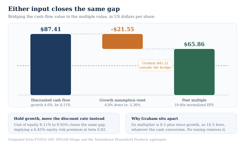
That gap resolves into two candidate inputs, each testable. Hold the cost of equity at 8.11 percent and terminal growth at 2.5 percent. The peer multiple is then consistent with explicit-period growth near negative 2.36 percent, against the 4.0 percent the filings recorded over 2021 to 2025. Five years of contraction followed by 2.5 percent in perpetuity is a diagnostic solve rather than a coherent forecast.

Hold growth at 4.0 percent and terminal growth at 2.5 percent instead, and the multiple implies a cost of equity near 9.93 percent. At a beta of 0.82 that is an equity risk premium of about 6.45 percent, against Damodaran's 4.23 percent. Holding the premium at 4.23 percent instead, it is an implied beta of about 1.25. The inversion cannot separate the two. This is a reverse DCF used as a reconciliation tool, not a standalone method.

Either statement is testable. Both published figures take the rounded 3.35 dollars and 8.11 percent through the arithmetic.

Where this leaves the analyst

The Graham output sits outside that bridge, and it should. Its distance is not an assumption that can be tuned. It comes from the multiplier's structure: 8.5 plus twice the growth input, scaled to about 12.6 times here by the bond-yield term. No channel exists through which cash conversion or capital intensity can enter. Treat the Graham output as a structural cross-check rather than a third estimate of the same quantity.

What survives is a valuation range of 42.22 to 87.41 dollars per share. The cash-flow and multiple methods sit between 65.86 and 87.41, and the Graham output sits below both for structural reasons, not as a judgment about value. The width says most of the answer depends on a growth path and a required return that the filings cannot settle. The range spans the three point outputs at base-case inputs. It is not a confidence interval. The cost-of-equity sensitivity above reaches 117.42 dollars at the favorable corner, and that width sits inside the discounted cash flow output alone. Constructing valuation ranges covers the wider framework this one sits in.

The residual width has a direct operational use. A wide span after verification means more of the estimate rests on judgment, and that argues for a larger margin of safety before any position is considered. A narrow span would mean the methods agree on the assumptions that matter, and would justify a smaller buffer.

The discipline that makes this repeatable is dull and non-negotiable. Normalize once and feed every method the same figures, then name the convention before reporting any output. Translate the disagreement into a single input where possible, and report the span.

Keeping the cash-flow side auditable is where tooling earns its place. The InvestViable Valuator runs a DCF from three explicit inputs: the cash flow growth path, the discount rate, and the terminal growth rate, every assumption user-controlled. The normalization itself is judgment applied to the filing, and it reaches the model the way every assumption does: through the inputs you set. The translation in the bridge above starts from assumptions you can read directly. For sector context, the consumer staples section of the Stock Universe ranks the sector's constituents by fundamentals and Investment Score. The stock screener applies the same filters across the market.

Run the next one the same way, and the ranges become comparable across companies. That comparability is what a multi-method stock valuation is for.