DCF Fade Period: How Growth, Margins and ROIC Converge

What is a DCF fade period, and where does it sit?

Many company valuations run in two stages: a few years forecast line by line, then a perpetuity that values everything after. That structure works when the business is already mature in the final forecast year. It fails when the explicit forecast ends with growth at 12 percent and returns far above the cost of capital. The perpetuity then capitalizes a business that does not yet exist.

The three-stage DCF fixes that by inserting a bridge. Stage one holds the near-term forecast. Stage two, the fade period, moves each driver from its stage-one level to its steady-state level. Stage three is the terminal value, computed on a business that has finished changing. The DCF methodology guide covers the first and third stages. This article builds the second.

Two neighboring articles own the rules on either side of the bridge, and this one does not repeat them. The DCF inputs checklist owns the terminal-value audit: the perpetual growth ceiling, the Gordon and exit-multiple cross-check, and the reinvestment test in the terminal year. Valuation sensitivity analysis owns how the answer moves when the perpetual growth rate or the discount rate is flexed. The fade is construction work that happens before either of those checks runs. It decides what the terminal year looks like when the audit begins.

The construction has a single objective. By the final explicit year, every driver should already sit at the value the terminal formula will use. If growth, margin or return on capital is still moving in that year, the perpetuity freezes a business in mid-transition and values the transition forever.

Which drivers converge, and to what targets?

Three drivers carry the fade. Each needs a target before the path toward it can be drawn.

Revenue growth converges to the perpetual growth rate the terminal value will use. Choosing that rate is terminal-value work, covered in the checklist. The fade's job is only to arrive there, from whatever growth the near-term forecast supports, without a cliff.

Operating margin converges to a level that competitors and customers will allow over the long run. The natural anchor is the margin of the industry the company will most resemble once it matures. Aswath Damodaran's margins by industry dataset, with data as of January 2026, shows how far those anchors sit apart. In his industry groupings, pre-tax unadjusted operating margin is 32.98 percent for system and application software and 6.80 percent for general retail. The figure is 13.14 percent for the US total market excluding financials. A margin target outside its industry's range needs a reason that can be written down.

Return on new invested capital converges toward the cost of capital, because excess returns attract competition. Where it settles is a judgment about durability. Setting it equal to the cost of capital means growth after the fade adds no value. Setting it above means the business keeps an edge in perpetuity, a claim the economic moat assessment is built to test. The discount rate and WACC guide covers the cost of capital itself.

These three are linked by reinvestment, so they cannot be set in isolation. A company growing faster, or earning less on each new dollar, must reinvest more. Return on new capital is also distinct from return on the existing base. ROIC versus ROE and ROA explains the return metric on reported figures. The fade uses the incremental version: what the next dollar of capital earns, which can be well below the average across older assets.

How long should the fade period run?

No rule sets the length. Evidence narrows it, and three kinds of evidence carry most of the weight.

The first is how rarely high growth lasts. Louis Chan, Jason Karceski and Josef Lakonishok studied long-term growth across a broad cross-section of US stocks. Their paper on the level and persistence of growth rates found very high growth to be rare and found little persistence beyond chance. They conclude that valuations assuming high growth over prolonged periods rest on shaky foundations. A long stage of high growth therefore needs company-specific evidence, not extrapolation.

The second is how quickly excess profitability erodes. Eugene Fama and Kenneth French estimated mean reversion in profitability at about 38 percent per year in a simple partial adjustment model. Their study of forecasting profitability and earnings also found reversion faster when profitability sits below its mean. A 38 percent annual closure implies a half-life of about 1.45 years, since 0.62 raised to 1.45 is close to one half. After five years, about 9 percent of the original gap would remain. That is a population average. It describes the typical firm, and the reason to model a longer fade is evidence that a company is not typical.

The third is the company's own durability case. An advantage with an end date, such as a patent term or a long contract, supplies a fade length directly. An advantage that compounds, such as a network effect, can justify a longer fade and a terminal return above the cost of capital. Name the source before assigning the years.

One more check is available from the market itself. A reverse DCF on today's price solves for the growth the price implies. Hold that growth and solve for the length instead, and you see the fade the market is already assuming. A model that needs a much longer fade than that is a claim that the market underrates durability. Write the claim down and gather the evidence for it.

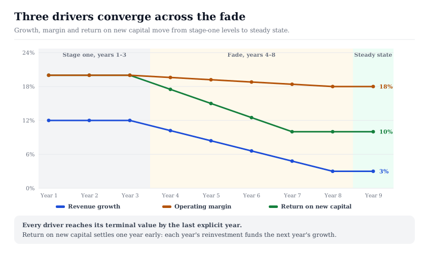
In practice, the fade ends when growth can reach the perpetual rate without a step and margins can reach their anchor. In the worked example below, a company growing at 12 percent reaches 3 percent over five years, in steps of 1.8 percentage points. Treat that length as an input to defend with the evidence above, not as a default.

Linear or geometric: which fade shape should you use?

Length decides when the drivers arrive. Shape decides how much of the excess survives along the way, and the two common shapes value the same endpoints differently.

A linear fade closes the gap in equal steps. Take a return on new capital of 20 percent fading to 10 percent over five years. The linear path runs 18, 16, 14, 12 and 10 percent. It is transparent, easy to audit, and lands exactly on the target in the final year. It assumes competition erodes the advantage at a constant pace in percentage points.

A geometric fade closes a fixed fraction of the remaining gap each year, which matches the partial adjustment idea behind the Fama and French estimate. At their 38 percent rate, the 10-point gap shrinks to 6.20, 3.84, 2.38, 1.48 and 0.92 points. The return path becomes 16.20, 13.84, 12.38, 11.48 and 10.92 percent. It front-loads the decline, so early fade years carry less excess return than the linear path gives them.

The geometric path has one practical defect: it never arrives. After five years it still sits 0.92 points above target, and the terminal formula would capitalize that residue forever. The fix is a snap rule. Set every driver to its target in the final fade year, whatever the curve says, and state that you did so.

Shape also has to be consistent across drivers. Fading growth linearly while dropping the return on new capital in one step produces years where the model invests heavily at a return it has already abandoned. Choose one convention, apply it to all three drivers, and record it next to the inputs. The dividend discount model guide prices the same step-versus-fade choice for a dividend stream. On its inputs, the linear fade returns less than the one-step model, because there the fade replaces years the step model holds at peak growth.

How to keep reinvestment consistent with growth

Reinvestment is where most fade periods break. A model fades growth to 3 percent but keeps capital spending at its stage-one share of revenue. The result is a mature company still investing like a fast grower, and cash flow understated for every remaining year. The opposite error, growth held high while reinvestment shrinks, overstates cash flow. Both disappear when reinvestment is derived rather than forecast.

The formula has a timing built into it. Capital invested this year produces next year's revenue, so this year's reinvestment depends on next year's growth. That has a consequence for the fade schedule. The return on new capital should reach its steady value one year before growth does. Capital invested in the year before growth reaches its perpetual rate funds the first year of steady-state growth, so it is already steady-state capital. In the worked example that is year 7, which funds year 8's 3 percent growth.

An equivalent form uses a sales-to-capital ratio: reinvestment equals next year's revenue increase divided by revenue generated per dollar of new capital. The return on new capital is then the after-tax margin times that ratio. Damodaran's capital expenditures by sector dataset reports the average sales-to-invested-capital ratio by industry, as of January 2026. That ratio describes the existing capital base, so use it as an anchor for the incremental ratio rather than as a direct measure. It shows 1.54 for system and application software, 1.21 for semiconductors and 3.51 for general retail. The US total market excluding financials sits at 1.43. Those figures are a sense check on the fade's endpoint: a steady-state ratio far outside the company's industry needs a reason.

Before the terminal value is applied, run one handoff test. In the final explicit year, the reinvestment rate should equal perpetual growth divided by the terminal return on new capital. If it does, the bridge and the perpetuity describe the same business. The checklist applies the same test from the terminal side; a well-built fade passes it by construction.

A worked fade: building the bridge year by year

The example is illustrative and every figure recomputes from the stated inputs. A company has revenue of 1,000 in year zero, a 25 percent tax rate and an 8.5 percent cost of capital. Stage one, years 1 to 3, holds growth at 12 percent, margin at 20 percent and return on new capital at 20 percent. The steady state is 3 percent growth, an 18 percent margin and a 10 percent return on new capital. The 10 percent terminal return sits 1.5 points above the cost of capital. Even the base case therefore assumes a small edge that lasts; setting the return to 8.5 percent would remove it.

The fade runs over years 4 to 8. Growth steps down by 1.8 points a year: 10.2, 8.4, 6.6, 4.8 and 3.0 percent. Margin eases by 0.4 points a year to 18.0 percent. Return on new capital falls by 2.5 points a year and reaches 10 percent in year 7, one year ahead of growth.

The reinvestment rate follows directly. It is 60 percent in years 1 and 2, 12 divided by 20, and 51 percent in year 3, where next year's growth is 10.2. It then runs 48, 44 and 38.4 percent in years 4 to 6. In year 7 it is 30 percent, which is 3 divided by 10. Year 8 repeats 30 percent and passes the handoff test. Free cash flow rises every year, from 67.2 in year 1 to 182.5 in year 8.

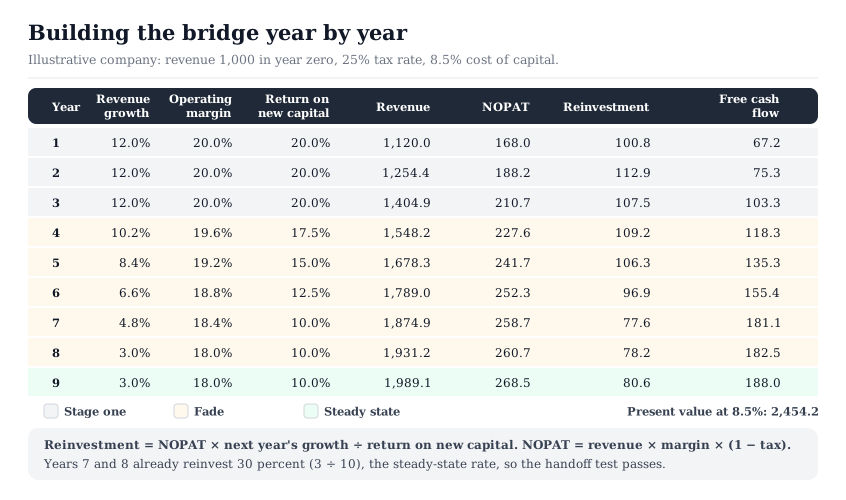
Discounted at 8.5 percent, the eight explicit cash flows are worth 674.7. Year 9 free cash flow is 188.0, which is NOPAT of 268.5 less 30 percent reinvestment. Capitalized at 8.5 minus 3 percent, it gives a terminal value of 3,417.6 at the end of year 8, worth 1,779.5 today. The total is 2,454.2. That figure is an output of these inputs, not an estimate for any real company.

Now change one decision at a time. Keep the same growth and margin path, but hold return on new capital at 20 percent forever. Reinvestment falls to 15 percent in the final years, and the value rises to 2,927.6, about 19 percent higher. Nothing in the growth path changed: the extra value is an unstated claim of a permanent edge. Next, skip the fade and step growth, margin and return to their steady-state values in year 4. The value falls to 2,212.7, about 10 percent lower. Here the fade extends stage one instead of replacing part of it, so the step returns less. Year 3 also shows a free cash flow spike to 179.1, because reinvestment drops ahead of the step.

Where the fade period fits in your workflow

The fade is built after the near-term forecast and before the terminal value is audited. Set the three steady-state targets first and write down where each comes from. Choose the length from the evidence on durability, then the shape, then snap every driver to its target by the final year. Derive reinvestment in every year from the formula above, and run the handoff test before the terminal formula touches the model. Then hand the terminal year to the DCF inputs checklist for its audit. The final step is a stress test of the drivers that dominate the value.

The worked example shows why this ordering matters. Its two variants moved value by about 19 and 10 percent without touching the perpetual growth rate. Neither change would show up in a terminal-value audit that checks only the final formula. The fade decides what the audit is checking.

When you test assumptions in the InvestViable Valuator, its inputs are the cash flow growth path, the discount rate and the terminal growth rate. Margin, reinvestment and return on capital are not separate inputs there; they live in your own bridge, and the cash flow path is what that bridge produces. A fade schedule kept beside the inputs makes the growth path auditable. Companies in the growth stocks slice of the Stock Universe are where the bridge carries the most weight, because their stage-one numbers sit furthest from steady state. Primary filings on SEC EDGAR supply the historical growth, margins and capital base that anchor the starting point.