Dividend Discount Model: When the DDM Still Applies

What the dividend discount model actually values

Every intrinsic valuation rests on the same claim: an asset is worth the present value of what it pays its owner. The dividend discount model is the most literal reading of that claim. The only cash a shareholder receives from simply holding a share is the dividend, so the dividend is what gets discounted. John Burr Williams put the argument in print in 1938, and the premise has not needed revision since. The closed forms that followed only changed how the tail gets handled.

The literalism is the whole design, and it cuts both ways. A cash flow model estimates what a business could distribute, which requires a judgment about reinvestment. A dividend model takes what the business does distribute, which requires no judgment at all about the payout, only about its future path. On a company whose board sets the dividend by policy and rarely deviates, that is a real advantage. You are forecasting a declared, auditable number rather than reverse-engineering one.

This is also an equity-side model, and the pairing matters. Dividends belong to shareholders alone, so they are discounted at the cost of equity, never at a blended cost of capital. Discounting a dividend at a weighted average cost of capital mixes a shareholder cash flow with a lender's required return, and the resulting value is too high. The discount rate and WACC walkthrough sets out how the cost of equity is built and where the blended rate legitimately belongs.

The DDM formula and the constraint on growth

The general form is a sum: the value of a share is each future dividend divided by one plus the cost of equity, raised to the year it arrives. Nobody forecasts an infinite series, so the practical DDM formula closes the tail with a perpetuity. In the single-stage case the entire model collapses into one line.

Value per share equals next year's dividend, divided by the cost of equity minus the perpetual growth rate.

Two conditions have to hold before that line means anything. The first is mechanical: growth must sit below the cost of equity, or the denominator turns negative and the model returns a negative price. The second is economic and binds much earlier. A company growing forever faster than the economy around it eventually becomes the economy. Damodaran's treatment of dividend discount models states the resulting cap plainly: the stable growth rate cannot exceed the growth rate of the economy in which the firm operates. For a US company that ceiling is long-run nominal growth. Take it from the nominal GDP series that FRED carries from the Bureau of Economic Analysis, and say which window you averaged.

Name the convention you are using. This is a perpetuity close, which assumes the dividend compounds at a fixed rate forever. The alternative is to end the forecast at an exit multiple and let a market price stand in for the tail. The two produce different answers, and quoting one without saying which you used hides the assumption doing most of the work.

The Gordon growth model on one stable payer

Take a company that just paid 2.00 per share in its reporting currency, growing at 3 percent, with a cost of equity of 8.5 percent. Next year's dividend is 2.06. Divide that by the 5.5-point spread between the discount rate and the growth rate and the Gordon growth model returns 37.45 per share.

Now move one input by a single point. Lower the cost of equity to 7.5 percent and the value rises to 45.78, up 22 percent. Raise the growth rate to 4 percent instead and the value reaches 46.22. Neither change alters the business. Both change the answer by more than a fifth, because the spread in the denominator is small and a one-point move is a large fraction of it.

A dividend growing forever has to be funded by retained earnings, so growth cannot exceed the retention rate times return on equity. At a 60 percent payout, 3 percent perpetual growth implies a return on equity of 7.5 percent. If the company earns materially less, the growth rate is being assumed rather than funded.

That fragility is the model's defining property, not a flaw to engineer away. It means the honest output is a range, not a figure. Run the calculation at both ends of a defensible cost of equity and report both values. The sensitivity analysis method covers how to build that table properly, and the discount you then demand below the range belongs to a separate discipline, the margin of safety.

Two stages, and where the value really sits

Not every dividend payer is already in a steady state, and the single-stage form is the wrong tool for the ones that are not. The standard repair is a two-stage model: forecast the dividend explicitly through a period of higher growth, then apply the perpetuity to what follows. A fade variant smooths the transition instead of stepping it down in one jump, and the H-model is the standard closed form for that linear decline.

Take the same 2.00 dividend, growing at 8 percent for five years and 3 percent thereafter, discounted at 8.5 percent. The five explicit dividends are 2.16, 2.33, 2.52, 2.72 and 2.94. Their present values sum to 9.86. The year-six dividend, 3.0268 before rounding, divided by the same 5.5-point spread gives a terminal value of 55.03. That is worth 36.60 discounted back five years. Total value is 46.46 per share.

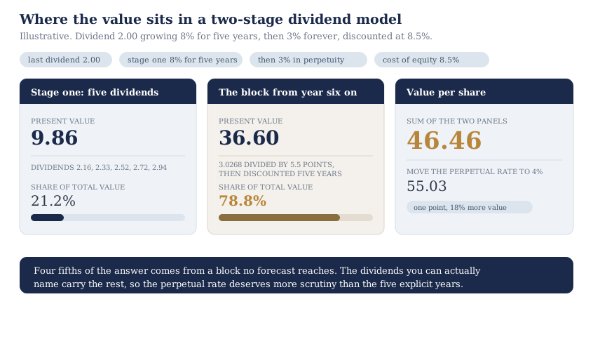
The five dividends you can actually name contribute 21.2 percent of the value. The remaining 78.8 percent comes from a perpetuity nobody can forecast. Move the perpetual rate from 3 to 4 percent and the total rises to 55.03. That figure coincidentally matches the terminal value above. It is an 18 percent gain from an assumption appearing once, in the model's last line. Analysts who spend their effort refining the explicit years are polishing a fifth of the answer.

The choice between a step and a fade is worth pricing too. On these same inputs the step model returns 46.46. A linear fade, stepping growth through 8, 6.75, 5.5, 4.25 and 3 percent before the perpetuity opens, returns 41.95. Stable growth from the first year returns 37.45. Holding peak growth flat for the full period is the least conservative of the three.

The test that decides whether the model applies

Run this check before any of the arithmetic above. Take the dividends the company pays and divide them by everything it returns to shareholders, dividends plus buybacks. If the ratio is near one, the dividend is the distribution and a dividend model is measuring the right thing. If the ratio is well below one, the model is valuing a fraction and treating the remainder as though it never happened.

Damodaran's dividend fundamentals dataset makes the spread visible across US industries.

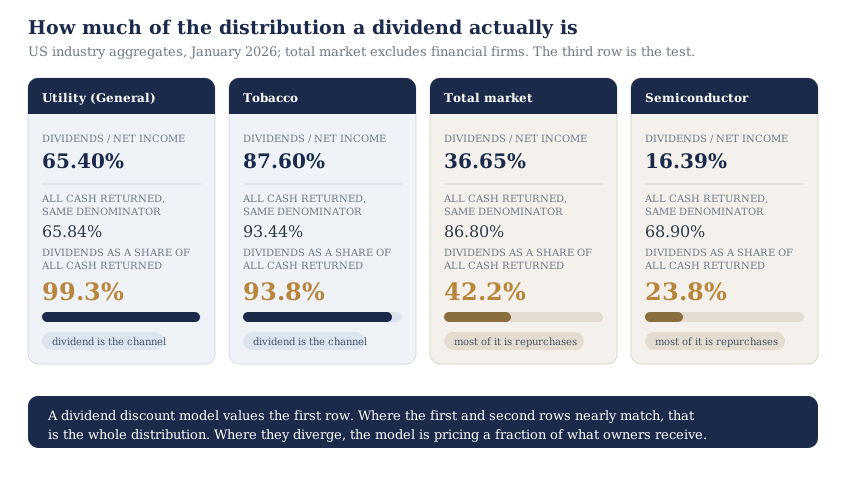
General utilities returned 65.84 percent of net income in total and paid 65.40 percent of it as dividends, so 99.3 percent of the distribution arrives as a dividend. The larger Power aggregate, 46 firms against 14, reads 97.1 percent on the same test, and Tobacco reaches 93.8 percent. Those are the industries where a dividend model is not an approximation of anything; it is the direct measurement. Across the total US market excluding financials, the same ratio is 42.2 percent, and in semiconductors it falls to 23.8 percent. Applying a dividend-only model to a semiconductor business values under a quarter of what shareholders receive. One qualification runs the other way. The buyback column comes from the cash flow statement, and some filers report it net of issuance while others do not. Part of a repurchase may only be offsetting dilution. Damodaran publishes the issuance-adjusted figure alongside it. Net of issuance the market's dividend share rises from 42.2 to 51.8 percent, and the semiconductor share from 23.8 to 26.0 percent. Neither move changes the verdict. General utilities travel the opposite way, to 201.8 percent, because net of issuance they return less cash than they pay in dividends.

Where repurchases dominate, two repairs work. Model the total payout, dividends plus buybacks, as the distribution being discounted. Or move to free cash flow to equity and value the cash the business could return, discounted at the same cost of equity. That is the approach the owner earnings comparison develops. The second is more robust, because a buyback program is discretionary in a way a declared dividend is not. Judging whether the repurchases themselves created value is a separate question, handled in the buyback analysis method.

Four ways the model breaks quietly

The loud failures are easy to catch: a negative denominator, or a company that pays nothing at all. These four are quieter.

The company does not pay yet. A company that will initiate a dividend in eight years technically has a dividend stream, and the framework will happily discount it. But the value then rests almost entirely on the date and size of a payout that does not exist yet. That is a guess wearing formula notation.

The payout ratio misreads the funding source. Real estate investment trusts paid dividends worth 194.87 percent of net income in the same January 2026 dataset. That is not distress; depreciation depresses reported earnings for property owners, and the distribution comes out of cash flow the income statement understates. But a payout ratio above one demands that you check which measure the dividend is actually funded from before extrapolating it.

The dividend is funded by borrowing or asset sales. A payout that free cash flow to equity does not cover is being financed, and financed dividends do not grow forever. This is a data-quality question before it is a valuation question. Verify the declared dividend and the cash flow behind it in the filings themselves through SEC EDGAR rather than a summary figure.

Policy is mistaken for capacity. A stable dividend tells you what the board chose, not what the business can afford. Those coincide at a mature utility. They diverge at a company holding its payout flat while earnings compound. A dividend model then understates value year after year, and looks consistent doing it.

Where a dividend model belongs in the workflow

Treat the DDM as a cross-check with a narrow domain, never as a primary engine. On a regulated utility or a mature staples business it can lead. The dividend is the distribution there, and the payout policy is the most predictable thing about the company. Everywhere else it earns its place as a second opinion, which is the multi-method discipline applied to one model. It reads cash actually paid, set beside a cash flow model reading cash potentially available. It is a floor only where free cash flow to equity covers the payout. Where the dividend is financed, it runs above the capacity figure rather than below it. When the two disagree, the gap is usually the reinvestment assumption, and that gap is more informative than either figure alone.

Banks are the structural case. For a lender, debt is raw material and not financing, so free cash flow to the firm has no clean definition. Free cash flow to equity is the other equity-side option. Regulatory capital requirements make a bank's reinvestment need hard to pin down, which pushes the declared payout back to the front. Run the payout-channel test on them anyway. Financials sit outside the market aggregate quoted above, and in the same January 2026 data money-center banks returned 44.0 percent of their distribution as dividends, regional banks 60.7 percent. Structural fit does not exempt a company from the test.

Telecom is the mirror case. Wireless operators returned 160.90 percent of net income in the same January 2026 data, and only 32.0 percent of that reached shareholders as dividends. Wireline telecom services runs the other way. An established payout history is not the test. The payout channel is.

The method-selection question comes first, and choosing the valuation method by company type works through the sequence. The stock valuation methods guide is the parent piece for the wider set of approaches. The Graham formula covers the other shorthand, which capitalizes earnings without discounting an explicit stream.

For the cross-check itself, the InvestViable Valuator runs a discounted cash flow from three explicit inputs: the cash flow growth path, the discount rate and the terminal growth rate. Every assumption stays user-controlled. Building the dividend model by hand alongside it is the whole comparison. The InvestViable stock screener filters the US universe on fundamentals. Stock Universe slices such as dividend stocks or dividend-paying utilities then narrow the field to the profile this model was built for.